OpenCV algorithms work best on rectangular frames. But when a camera is deployed on a real road, it is very hard to position the camera so that the road to be monitored is a perfect rectangle, and the camera gets a top view of that rectangle. Typically the road to be monitored is at an arbitrary angle to the camera, and many additional objects are part of the frame. For useful tasks like traffic density estimation on a particular road stretch, it is therefore important to first correct the camera angle in software, and crop the image to remove the additional objects. This is the goal of the first assignment Subtask1.
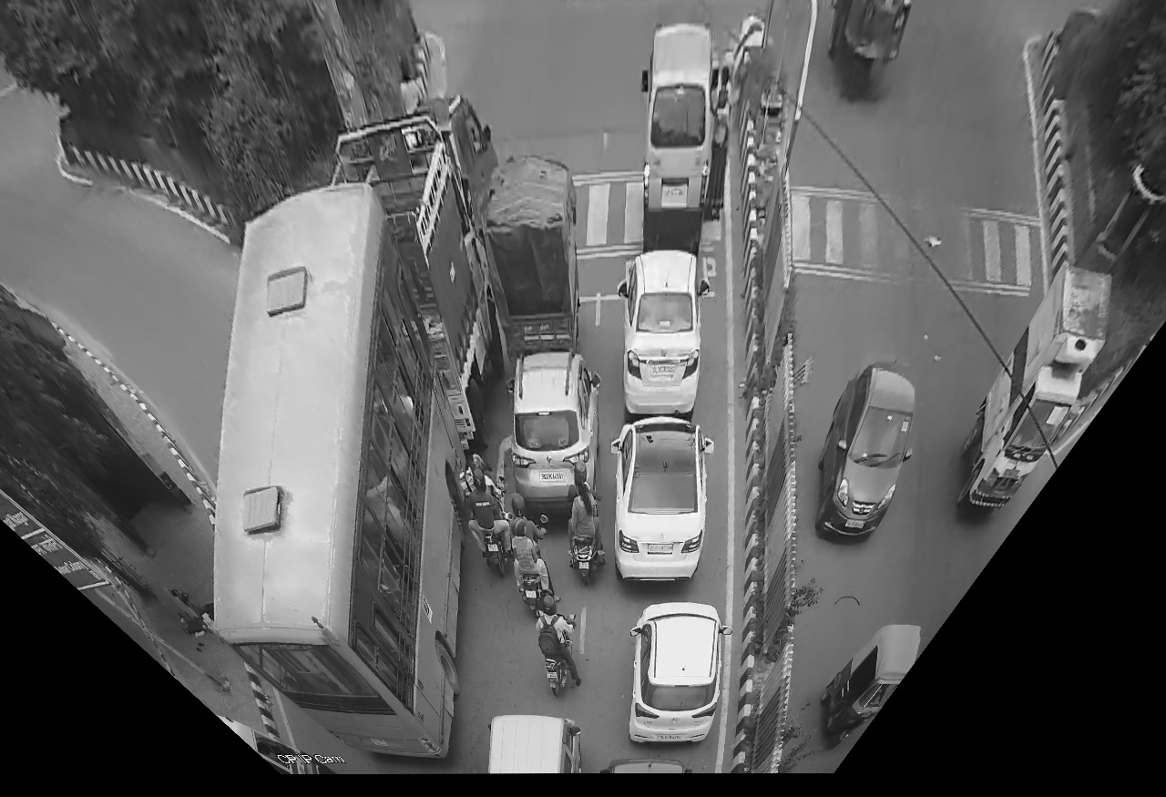
The images above show two frames from a traffic camera in Lajpatnagar junction in New Delhi, the first without and the second with vehicles. Suppose we will estimate the density of traffic in Subtask2, for vehicles which are waiting for red signal in the straight stretch of the road going towards north. The camera does not have a top view of this stretch (see the divider which indicates that the camera is not perpendicular to the road). There are also many additional objects in view of the camera (the divider, the road in the opposite direction, road beyond the zebra crossing, road going to the west etc.). You can get these two images at empty.jpg and traffic.jpg respectively. Use these two images in your code, for camera angle correction and cropping. Tutorial1, tutorial2 are two relevant tutorials that use OpenCV functions for camera angle correction.
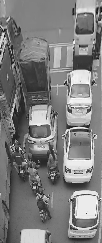
The images above are the projected and cropped images (in grayscale) of the original images respectively. Your code should take the given two input images and produce similar outputs. We say "similar" and not "exact same", because the angle correction will depend on your manual selection of four points on the original frames, and this manual selection might vary from person to person, and also for the same person across different runs. The video shows how Riju's implementation takes the manual inputs of the four corners of the straight road going towards north, using mouse clicks. You will need to implement similar logic to take your mouse click inputs, and then use those coordinates for angle correction. Riju uses (472,52),(472,830),(800,830),(800,52) as the second set of points, where her mouse-clicked points get mapped during angle correction. You can also use these values as your second set of points.

We will create an assignment in Moodle. Any one of the two team members upload a single tar file there with name entrynum1_entrynum2_ass1_part1.tar.gz. It should contain your source code, Makefile and a readme describing how to run your executable from command line. E.g. command line ./yourcode.out empty or ./yourcode.out traffic. A wrong command line should print the appropriate help. Your code should take the mouse inputs and show the transformed and cropped frames (as in the video). It should also save the transformed and cropped frames as jpg files in the same folder.

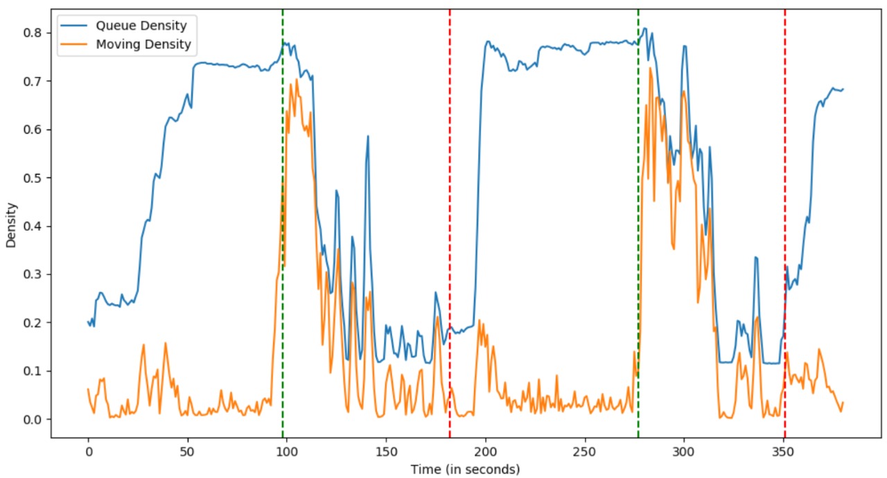
Below is a video from Lajpatnagar junction. Your submitted code should take such a video as input. The output should be queue density (blue line in the graph below) and dynamic density (orange line) for the video frames. Queue density is density of all vehicles queued (either standing or moving) which are waiting for red signal in the straight stretch of road going towards north (output after angle correction and cropping in Subtask1). Dynamic density is the density of those vehicles which are not standing but moving in that same stretch. The vertical lines in the graph show when the signal turned green or red in this particular video clip for the road stretch under consideration. After the green vertical line (when signal turns green), the dynamic density instantly peaks (as all vehicles start moving) and the queue density starts coming down (the queue of waiting traffic gradually gets cleared). After the red vertical line (when signal turns red), the dynamic density drops (as vehicles can't move now), while the queue density starts to increase to saturation (as more and more vehicles accumulate). Use OpenCV functions as needed to compute the queue and dynamic densities. Queue density might need background subtraction, where you can pick the background frame as any empty frame from this video clip itself, or the empty frame from the same camera view given in Subtask1. Dynamic density might need optical flow across subsequent frames, to detect which pixels moved across frames. You will also need your code in Subtask1 for angle correction and cropping on every frame. Plot the ouput values against time and compare with the given graph. The output might not match in absolute values with the given graph(due to difference in parameters passed to the OpenCV functions), but the patterns (which curve comes down vs. which goes up) correspinding to signal changes should hold.

Again one of the two team members upload a single tar file there with name entrynum1_entrynum2_ass1_part2.tar.gz. It should contain your source code, Makefile and a readme describing how to run your executable from command line. E.g. command line ./yourcode.out videoname. A wrong command line should print the appropriate help. Your code should output three columns of values - "time (in secs), queue density, dynamic density" in command line when run, such that the TA can easily plot column 1 vs. column 2 (blue curve) or clumn 1 vs. column 3 (orange curve). Also include the output you got on your machine as out.txt and the correponding graph as an image, in the tar. The given video is 15 FPS. You can process every 3rd frame (processing at 5 FPS) or every 5th frame (processing at 3 FPS), if your laptop takes too much time to run your code on the 6 minute video.

When we build software, accuracy of the output or utility might not be the only metric to optimize. Sure, if we are estimating traffic density on road, we should output the correct density values. But maybe latency is also an important metric, that for a given input frame, we get output within a small time. Maybe throughput is an important metric, that every unit time, the code generates high number of outputs. Maybe keeping the processor temperature under control is necessary, if the software is deployed on a roadside embedded board, where there is no AC and ambient temperatures in Delhi shoots to 45 degree Celsius in summer. Maybe energy is an important metric, if the roadside embedded board is solar-powered, and can generate only a limited amount of energy. Maybe we want to protect the software from hackers, and therefore security is vital too.

These metrics might be at conflict with each other. E.g. for higher throughput, processors might run at a higher frequency, thereby draining more power and heating up more. Putting security checks against hackers might make the code run slower. This aspect of having multiple metrics to optimize, which conflict with each other, is called trade-off. Software design might need careful trade-off analyses.

In addition to metrics, we have to understand three more terms (i) benchmark, (ii) baseline, and (iii) methods/parameters, for trade-off analysis. Benchmark is the dataset on which we analyze the trade-offs. The video that we used for Assignment 1 part(b), can be benchmark for Assignment 1 part(c). Baseline is the method against which we compare other methods/parameters, and see whether we are getting a better or worse trade-off. Your Assignment 1 part(b) code can be your baseline for Assignment 1 part(c). Finally methods/parameters are software variants, which we compare against the baseline method, to see whether trade-off improves or degrades.

In Assignment 1 part(c) we will do an utility-runtime tradeoff analysis for queue density estimation (using background subtraction). You need to define your utility metric --- maybe the difference in queue per unit time, compared to baseline, take the absolute or squared value of that as error. The lower this error, the higher is your utility. You can take the average/median of that error over the whole video, to get a single value for utility. Similarly for runtime, you can take the time for processing the whole video. You can have a plot, where x-axis is utility and y-axis is runtime, and different points in that plot will come from different methods/parameters.

For this task's utility-runtime trade-off analysis, we can have the following methods/parameters (All based on background subtraction for queue density only, and no optical flow. Optical flow for dynamic density is mentioned below in extra credit.):

• Method1: sub-sampling frames -- processing every x frame i.e. process frame N and then frame N+x, and for all intermediate frames just use the value obtained for N - total processing time will reduce, but utility might decrease as intermediate frames values might differ from baseline. Parameter for this method is x, how many frames you drop.
• Method2: reduce resolution for each frame. Lower resolution frames might be processed faster, but having higher errors. Parameter can be resolution XxY.
• Method3: split work spatially across threads (application level pthreads) by giving each thread part of a frame to process. Parameter can be number of splits i.e. number of threads, if each thread gets one split. You might need to take care of boundary pixels that different threads process for utility.
• Method4: split work temporally across threads (application level pthreads), by giving consecutive frames to different threads for processing. Parameter can be number of threads.

You have to submit on March 31, but working regularly with intermediate deadlines might help. For example:

• March 11 - March 18 [multi-threading methods]: Try to implement Method3 and Method4 above, learning about pthreads. See whether you can match your current single threaded output, using multiple threads.
• March 19 - March 25 [other methods]: Try to implement Method1 and Method2.
• March 26 - March 31 [plotting, analysis and report writing]: Plot utility vs. runtime for the four methods and parameters you choose. Create a latex report on overleaf with three sections -- I. Metrics (define your utility and runtime metrics here), II. methods (describe what methods you could implement from the above list with what parameters) and III. trade-off analysis (put tables and graphs and describe which method gave what utility-vs-runtime trade-off and why do you think it behaved in certain ways). To understand multi-threading behavior, you might need some command line tools like top or perf, to see your CPU and memory usage.

Extra Credit: If you implemented dynamic density in part(b) using optical flow, you can additionally compare sparse vs. dense optical flow for dynamic density, where baseline is dense optical flow based. Sparse might be faster, but have errors compared to dense. Relevant tutorials: tutorial
What to submit: Make two folders "code" and "analysis". The "code" folder should have as usual you cpp, headerfiles, Makefile and readme (on how to run your code). The "analysis" folder should have your code output files, post-processing scripts if any (e.g. to sort frames output in random order by different threads, to compute the utility value using two output files etc.), plotting scripts and the PDF report. A readme file in the "analysis" folder should include a description of all files (outout and scripts). Have sub-folders if that helps you organize things better. Remember that this is a design course, so the quality of your graphs and reports, depth of your analysis, cleanliness of your code, code organization and Makefile --- all are as important as code correctness. Even if you cannot implement all methods correctly, put efforts in the plot, analysis, writing report of the methods you can implement. Put "code" and "analysis" folders in entrynum1_entrynum2_ass1_part3.tar.gz and upload on Moodle.

This can be Pacman kind of maze game where the two players compete in time taking turn alternately in playing pacman or play simultaneously in side by side separate screens. Think of a way to give points to the players and a win/loss criteria. Or maybe one player controls pacman and the other player moves around the monsters trying to block pacman until a timeout. Generate a new random maze for each gameplay, so that the players don't get used to the maze structure on multiple games and get bored. This is just a sample 2 player maze game. You can think of your own game using a maze and build it.

Focus on cool and fun look of the game. Smooth controls. Appropriate message when network between the players is slow. Use sound effects. Bonus points if you come up with your own 2 player maze game to build instead of 2 player pacman. Minimum requirement for non 0 marks: single player pacman which is not copied from Internet.

What to submit:There will be no Moodle submission link for this. You need to commit everything on git by May 19 11:59 pm. Any commit after that will be ignored. What we will check on git: (a) The source code of the game with cpp, header and Makefile. (b) Readme with installation instructions you used on your machine for different libraries and packages (with your OS details). Also all online resource links that you used to learn and get ideas from. (c) A status.txt file with status of the game at time of submission: if it compiles and runs as you want it, just mention that. But if you got stuck somewhere, like sockets didn't work for you or one of the I/Os (mouse or keyboard) gave issues that you couldn't resolve till the end, include the problem and whatever you tried. We will mark you for your efforts, even if things haven't all worked for you. (d) 10-15 slides in PDF format describing your game rules, game stages (with screenshot images) -- so that people who would like to play has a clear idea what to expect during the play. In demo, you will need to clone your own repo on your machine, build it using your Makefile and play the game, while sharing screen with the TA. The TA will ask you about the game logic, if you needed to maintain any state of the game to remember which player has done what, whether a few variables sufficed or you needed some data structure(s), what was your maze generation logic, what different functions in your code do.

Remember the COL106 endsem question where the largest possible Ironman droid had to reach T from S in a maze? The algorithm you wrote, if implemented, could have simulated the droid's movement in the maze. Simulation of real world events is an important task of computers, and this subtask needs you to simulate something in a maze environment. You can modify the COL106 major problem -- e.g. create a maze and place the 6 infinity stones in different locations. A droid has not only to reach from S to T, but also pick all the stones on its route. Think of the algorithmic changes you might need to visit the stones. The shortest path from S to T might not include the places containing the stones. After picking a particular stone your droid might need to backtrack, as the way ahead after the stone is a deadend. If you define your maze as a graph, then visiting all nodes in the graph is called Traveling Salesman Problem (TSP). Visiting a subset of nodes in the graph (the stone locations) is called Steiner TSP, and the special nodes Steiner nodes. Think/read whether you can optimally solve this problem, and if not then what heuristic will you use? Also can your droid see the whole maze at all times? Or is it only seeing in first person based on its current location? This is just a sample computer simulation. You can think of your own problem using a maze and solve it algorithmically.

Focus on algorithmically interesting mapping of the simulation. Try to understand correctness and runtime if possible. Write a latex report describing your simulation: what you would simulate, the algorithm (with links to online resources that you might have used to come up with the algorithm), runtime analysis, how would the simulation look (you can create some images of the envisioned simulation in ppt/pen-and-paper drawing and incllude those. Mention extra points you would consider like putting appropriate delays so that the animation is aesthetic to watch, what data structures you might need to implement your algorithm. The design document should be such that someone can pick up your plan for SURA this summer and start writing code to implement it.

What to submit: A latex report in PDF format with simulation design, as discussed above. On Moodle. Few students who have already implemented this, make your last git commit on May 21 and let your TA know for bonus points.