Lab-6: Part-A (Wrangling Files)
(Intro. to Data Science: IIT Delhi - Abu Dhabi)
Before you can work with data in Python, it helps to understand the files that store the source of the data. You want answers to a couple of basic questions:
- How much data do you have?
- How is the source file formatted?
Answers to these questions can be very helpful. For example, if your file is too large or is not formatted the way you expect, you might not be able to properly load it into a dataframe.
Although many types of structures can represent data, in this course, we primarily work with data tables, such as Pandas DataFrames and SQL relations. We focus on data tables for several reasons. Research on how to store and manipulate data tables has resulted in stable and efficient tools for working with tables. Plus, data in a tabular format are close cousins of matrices, the mathematical objects of the immensely rich field of linear algebra. And of course, data tables are quite common.
In this Lab, we introduce typical file formats and encodings for plain text, describe measures of file size, and use Python tools to examine source files. Later in the chapter, we introduce an alternative approach for working with files: the shell interpreter. Shell commands give us a programmatic way to get information about a file outside the Python environment, and the shell can be very useful with big data. Finally, we check the data table's shape (the number of rows and columns) and granularity (what a row represents). These simple checks are the starting point for cleaning and analyzing our data.
We first provide brief descriptions of the datasets that we use as examples throughout this Lab.
A.1 Data Source Examples
We have selected two examples to demonstrate file wrangling concepts: a government survey about drug abuse; and administrative data from the San Francisco Department of Public Health about restaurant inspections.
A.1.1 Drug Abuse Warning Network (DAWN) Survey
DAWN is a national health-care survey that monitors trends in drug abuse. The survey aims to estimate the impact of drug abuse on the USA's health-care system, and improve how emergency departments monitor substance abuse crises. DAWN was administered annually from 1998 through 2011 by the Substance Abuse and Mental Health Services Administration (SAMHSA). In 2018, due in part to the opioid epidemic, the DAWN survey was restarted. In this example, we look at the 2011 data, which have been made available through the SAMHSA Data Archive.
The target population consists of all drug-related emergency room visits in the US. These visits are accessed through a frame of emergency rooms in hospitals (and their records). Hospitals are selected for the survey through probability sampling, and all drug-related visits to the sampled hospital's emergency room are included in the survey. All types of drug-related visits are included, such as drug misuse, abuse, accidental ingestion, suicide attempts, malicious poisonings, and adverse reactions. For each visit, the record may contain up to 16 different drugs, including illegal drugs, prescription drugs, and over-the-counter medications.
The source file for this dataset is an example of fixed-width formatting that requires external documentation, like a codebook, to decipher. Also, it is a reasonably large file, and so motivates the topic of how to find a file's size. And the granularity is unusual because an ER visit, not a person, is the subject of investigation.
The San Francisco restaurant files have other characteristics that make them a good example for this Lab.
A.1.2 San Francisco Restaurant Food Safety
The San Francisco Department of Public Health routinely makes unannounced visits to restaurants and inspects them for food safety. The inspector calculates a score based on the violations found and provides descriptions of the violations. The target population here is all restaurants in San Francisco. These restaurants are accessed through a frame of restaurant inspections that were conducted between 2013 and 2016. Some restaurants have multiple inspections in a year, and not all of the 7,000+ restaurants are inspected annually.
Food safety scores are available through the city's Open Data initiative, called DataSF. DataSF is one example of city governments around the world making their data publicly available; the DataSF mission is to "empower the use of data in decision making and service delivery" with the goal of improving the quality of life and work for residents, employers, employees, and visitors.
San Francisco requires restaurants to publicly display their scores (see figure below for an example placard).
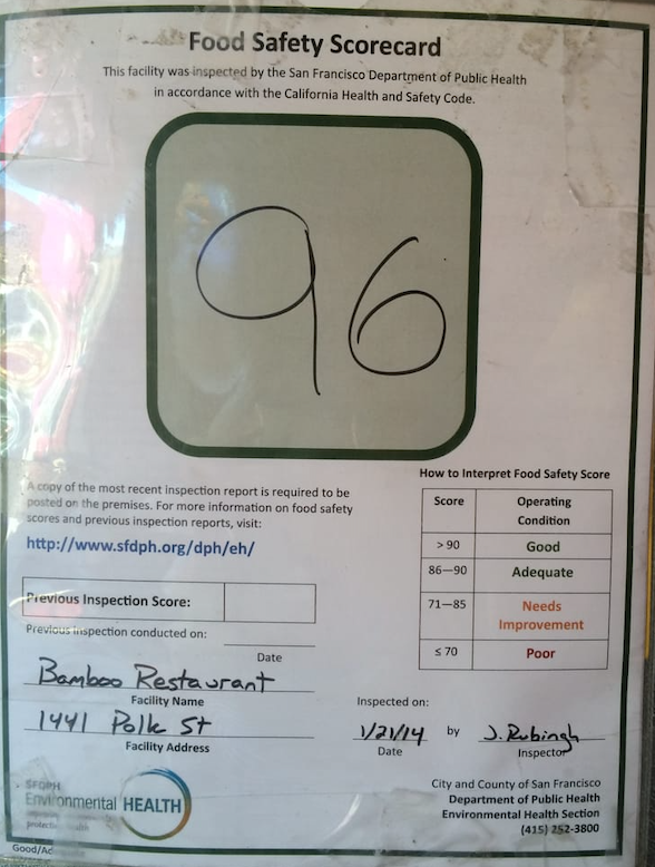 (A food safety scorecard displayed in a restaurant; scores range between 0 and 100)
These data offer an example of multiple files with different structures, fields, and granularity. One dataset contains summary results of inspections, another provides details about the violations found, and a third contains general information about the restaurants. The violations include both serious problems related to the transmission of foodborne illnesses and minor issues such as not properly displaying the inspection placard.
Both the DAWN survey data and the San Francisco restaurant inspection data are available online as plain-text files. However, their formats are quite different, and in the next section, we demonstrate how to figure out a file format so that we can read the data into a dataframe.
A.2 File Formats
A file format describes how data are stored on a computer's disk or other storage device. Understanding the file format helps us figure out how to read the data into Python in order to work with it as a data table. In this section, we introduce several popular formats used to store data tables. These are all plain-text formats, meaning they are easy for us to read with a text editor like VS Code, Sublime, Vim, or Emacs.
Note: The file format and the structure of the data are two different things. We consider the data structure to be a mental representation of the data that tells us what kinds of operations we can do. For example, a table structure corresponds to data values arranged in rows and columns. But the same table can be stored in many different types of file formats.
The first format we describe is the delimited file format.
A.2.1 Delimited Format
Delimited formats use a specific character to separate data values. Usually, these separators are either a comma (comma-separated-values, or CSV for short), a tab (tab-separated values or TSV), whitespace, or a colon. These formats are natural for storing data that have a table structure. Each line in the file represents a record, which is delimited by newline (\n or \r\n) characters. And within a line, the record's information is delimited by the comma character (,) for CSV or the tab character (\t) for TSV, and so on. The first line of these files often contains the names of the table's columns/features.
The San Francisco restaurant scores are stored in CSV-formatted files. Let's display the first few lines of the inspections.csv file. In Python, the built-in pathlib library has a useful Path object to specify paths to files and folders that work across platforms. This file is within the data folder, so we use Path() to create the full pathname:
from pathlib import Path

# Create a Path pointing to our data file
insp_path = Path() / 'data' / 'inspections.csv'
Note: Paths are tricky when working across different operating systems (OSs). For instance, a typical path in Windows might look like C:\files\data.csv, while a path in Unix or macos might look like ~/files/data.csv. Because of this, code that works on one OS can fail to run on other OSs.
The
pathlibPython library was created to avoid OS-specific path issues. By using it, the code shown here is more portable---it works across Windows, macos, and Unix.
The Path object in the following code has many useful methods, such as read_text(), which reads in the entire contents of the file as a string:
text = insp_path.read_text()
# Print first five lines
print('\n'.join(text.split('\n')[:5]))
"business_id","score","date","type"
19,"94","20160513","routine"
19,"94","20171211","routine"
24,"98","20171101","routine"
24,"98","20161005","routine"
Notice that the field names appear in the first line of the file; these names are comma separated and in quotes. We see four fields: the business identifier, the restaurant's score, the date of the inspection, and the type of inspection. Each line in the file corresponds to one inspection, and the ID, score, date, and type values are separated by commas. In addition to identifying the file format, we also want to identify the format of the features. We see two things of note: the scores and dates both appear as strings. We will want to convert the scores to numbers so that we can calculate summary statistics and create visualizations. And we will convert the date into a date-time format so that we can make time-series plots. We show how to carry out these transformations in a later lab.
Displaying the first few lines of a file is something we'll do often, so we create a function as a shortcut:
def head(filepath, n=5, width=-1):
    '''Prints the width characters of first n lines of filepath'''
    with filepath.open() as f:
        for _ in range(n):
            (print(f.readline(), end='') if width < 0
             else print(f.readline()[:width]))
Note: People often confuse CSV and TSV files with spreadsheets. This is in part because most spreadsheet software (like Microsoft Excel) will automatically display a CSV file as a table in a workbook. Behind the scenes, Excel looks at the file format and encoding just like we've done in this section. However, Excel files have a different format than CSV and TSV files, and we need to use different
pandasfunctions to read these formats into Python.
All the restaurant source files are CSV formatted. In contrast, the DAWN source file has a fixed-width format. We describe this kind of formatting next.
A.2.2 Fixed-Width Format
The fixed-width format (FWF) does not use delimiters to separate data values. Instead, the values for a specific field appear in the exact same position in each line. The DAWN source file has this format. Each line in the file is very long. For display purposes, we only show the first few characters from the first five lines in the file:
dawn_path = Path() / 'data' / 'DAWN-Data.txt'
head(dawn_path, width=65)
     1 2251082    .9426354082   3 4 1 2201141 2 865 105 1102005 1
     2 2291292   5.9920106887   911 1 3201134 12077  81  82 283-8
     3 7 7 251   4.7231718669   611 2 2201143 12313   1  12  -7-8
     410 8 292   4.0801470012   6 2 1 3201122 1 234 358  99 215 2
     5 122 942   5.1777093467  10 6 1 3201134 3 865 105 1102005 1
Notice how the values appear to align from one row to the next. For example, there is a decimal point in the same position (the 19th character) in each line. Notice also that some of the values seem to be squished together, and we need to know the exact position of each piece of information in a line in order to make sense of it. SAMHSA provides a 2,000-page codebook with all of this information, including some basic checks, so that we can confirm that we have correctly read the file. For instance, the codebook tells us that the age field appears in positions 34–35 and is coded in intervals from 1 to 11. The first two records shown in the preceding code have age categories of 4 and 11; the codebook tells us that a 4 stands for the age bracket "6 to 11" and 11 is for "65+."
Note: A widely adopted convention is to use the filename extension, such as .csv, .tsv, and .txt, to indicate the format of the contents of the file. Filenames that end with .csv are expected to contain comma-separated values, and those ending with .tsv are expected to contain tab-separated values; .txt generally denotes plain text without a designated format. However, these extension names are only suggestions. Even if a file has a .csv extension, the actual contents might not be formatted properly! It's a good practice to inspect the contents of the file before loading it into a dataframe. If the file is not too large, you can open and examine it with a plain-text editor. Otherwise, you can view a couple of lines using
.readline()or shell command.
Other plain-ext formats that are popular include hierarchical formats and loosely formatted text (in contrast to formats that directly support table structures). These are covered in greater detail in other chapters, but for completeness, we briefly describe them here.
A.2.3 Hierarchical Formats
Hierarchical formats store data in a nested form. For instance, JavaScript Object Notation (JSON), which is commonly used for communication by web servers, includes key-value pairs and arrays that can be nested, similar to a Python dictionary. The XML and HTML are other common formats for storing documents on the internet. Like JSON, these files also have a hierarchical, key-value format. We will cover both formats (JSON and XML) in more detail in a subsequent lab.
Next, we briefly describe other plain-text files that don't fall into any of the previous categories but still have some structure to them that enables us to read and extract information.
A.2.4 Loosely Formatted Text
Web logs, instrument readings, and program logs typically provide data in plain text. For example, here is one line of a web log (we've split it across multiple lines for readability). It contains information such as the date, time, and type of request made to a website:
169.237.46.168 - -
[26/Jan/2004:10:47:58 -0800]"GET /stat141/Winter04 HTTP/1.1" 301 328
"http://anson.ucdavis.edu/courses"
"Mozilla/4.0 (compatible; MSIE 6.0; Windows NT 5.0; .NET CLR 1.1.4322)"
There are organizational patterns present, but not in a simple delimited format. This is what we mean by "loosely formatted." We see that the date and time appear between square brackets, and the type of request (GET in this case) follows the date-time information and appears in quotes.
As another example, here is a single record taken from a wireless device log. The device reports the timestamp, the identifier, its location, and the signal strengths that it picks up from other devices. This information uses a combination of formats: key-value pairs, semicolon-delimited values, and comma-delimited values:
t=1139644637174;id=00:02:2D:21:0F:33;pos=2.0,0.0,0.0;degree=45.5;
00:14:bf:b1:97:8a=-33,2437000000,3;00:14:bf:b1:97:8a=-38,2437000000,3;
Like with the web logs, we can use string manipulation and the patterns in the records to extract features into a table.
We have primarily introduced formats for plain-text data that are widely used for storing and exchanging tables. The CSV format is the most common, but others, such as tab-separated and fixed-width formats, are also prevalent. And, there are many types of file formats that store data!
So far, we have used the term plain text to broadly cover formats that can be viewed with a text editor. However, a plain-text file may have different encodings, and if we don't specify the encoding correctly, the values in the dataframe might contain gibberish. We give an overview of file encoding next.
A.3 File Encoding
Computers store data as sequences of bits: 0s and 1s.
Character encodings, like ASCII, tell the computer how to translate between bits and text.
For example, in ASCII, the bits 01000001 stand for the letter A and 01000010 for B.
The most basic kind of plain text supports only standard ASCII characters, which
includes the uppercase and lowercase English letters, numbers, punctuation symbols, and spaces.
ASCII encoding does not include a lot of special characters or characters from other languages. Other, more modern character encodings have many more characters that can be represented. Common encodings for documents and web pages are Latin-1 (ISO-8859-1) and UTF-8. UTF-8 has over a million characters and is backward compatible with ASCII, meaning that it uses the same representation for English letters, numbers, and punctuation as ASCII.
When we have a text file, we usually need to figure out its encoding. If we choose the wrong encoding to read in a file, Python either reads incorrect values or throws an error. The best way to find the encoding is by checking the data's documentation, which often explicitly says what the encoding is.
When we don't know the encoding, we have to make a guess. The chardet package has a function called detect() that infers a file's encoding. Since these guesses are imperfect, the function also returns a confidence between 0 and 1. We use this function to look at the files from our examples:
import chardet

line = '{:<25} {:<10} {}'.format

# for each file, print its name, encoding & confidence in the encoding
print(line('File Name', 'Encoding', 'Confidence'))

for filepath in Path('data').glob('*'):
    with open(filepath, 'rb') as f:
        result = chardet.detect(f.read(1000000))
        print(line(str(filepath), result['encoding'], result['confidence']))
File Name                 Encoding   Confidence
data/inspections.csv      ascii      1.0
data/co2_mm_mlo.txt       ascii      1.0
data/violations.csv       ascii      1.0
data/DAWN-Data.txt        ascii      1.0
data/legend.csv           ascii      1.0
data/businesses.csv       ISO-8859-1 0.73
The detection function is quite certain that all but one of the files are ASCII encoded. The exception is businesses.csv, which appears to have an ISO-8859-1 encoding. We run into trouble if we ignore this encoding and try to read the business file into pandas without specifying the special encoding:
# naively reads file without considering encoding
>>> pd.read_csv('data/businesses.csv')
[...stack trace omitted...]
UnicodeDecodeError: 'utf-8' codec can't decode byte 0xd1 in
position 8: invalid continuation byte
To successfully read the data, we must specify the ISO-8859-1 encoding:
import pandas as pd

data =pd.read_csv('data/businesses.csv', encoding = 'ISO-8859-1')
data.iloc[:4, [0,1,2,5]]
| business_id | name | address | postal_code | |
|---|---|---|---|---|
| 0 | 19 | NRGIZE LIFESTYLE CAFE | 1200 VAN NESS AVE, 3RD FLOOR | 94109 |
| 1 | 24 | OMNI S.F. HOTEL - 2ND FLOOR PANTRY | 500 CALIFORNIA ST, 2ND FLOOR | 94104 |
| 2 | 31 | NORMAN'S ICE CREAM AND FREEZES | 2801 LEAVENWORTH ST | 94133 |
| 3 | 45 | CHARLIE'S DELI CAFE | 3202 FOLSOM ST | 94110 |
File encoding can be a bit mysterious to figure out, and unless there is metadata that explicitly gives us the encoding, guesswork comes into play. When an encoding is not 100% confirmed, it's a good idea to seek additional documentation.
Another potentially important aspect of a source file is its size. If a file is huge, then we might not be able to read it into a dataframe. In the next section, we discuss how to figure out a source file's size.
A.4 File Size
Computers have finite resources. You have likely encountered these limits firsthand if your computer has slowed down from having too many applications open at once. We want to make sure that we do not exceed the computer's limits while working with data, and we might choose to examine a file differently depending on its size. If we know that our dataset is relatively small, then a text editor or a spreadsheet can be convenient for looking at the data. On the other hand, for large datasets, a more programmatic exploration or even distributed computing tools may be needed.
In many situations, we analyze datasets downloaded from the internet. These files reside on the computer's disk storage. In order to use Python to explore and manipulate the data, we need to read the data into the computer's memory, also known as random access memory (RAM). All Python code requires the use of RAM, no matter how short the code is. A computer's RAM is typically much smaller than its disk storage. For example, one computer model released in 2018 had 32 times more disk storage than RAM. Unfortunately, this means that data files can often be much bigger than what is feasible to read into memory.
Both disk storage and RAM capacity are measured in terms of bytes (eight 0s and 1s). Roughly speaking, each character in a text file adds one byte to a file's size. To succinctly describe the sizes of larger files, we use the prefixes described in the table below. For example, a file containing 52,428,800 characters takes up $5,242,8800 / 1,024^2 = 50~{\textrm{mebibytes}}$, or 50 MiB on disk.
| Multiple | Notation | Number of bytes |
|---|---|---|
| Kibibyte | KiB | 1,024 |
| Mebibyte | MiB | 1,024² |
| Gibibyte | GiB | 1,024³ |
| Tebibyte | TiB | 1,024⁴ |
| Pebibyte | PiB | 1,024⁵ |
Note: Why use multiples of 1,024 instead of simple multiples of 1,000 for these prefixes? This is a historical result of the fact that most computers use a binary number scheme where powers of 2 are simpler to represent ($1,024 = 2^{10}$). You also see the typical SI prefixes used to describe size---kilobytes, megabytes, and gigabytes, for example. Unfortunately, these prefixes are used inconsistently. Sometimes a kilobyte refers to 1,000 bytes; other times, a kilobyte refers to 1,024 bytes. To avoid confusion, we stick to kibi-, mebi-, and gibibytes, which clearly represent multiples of 1,024.
It is not uncommon to have a data file happily stored on a computer that will overflow the computer's memory if we attempt to manipulate it with a program. So we often begin our data work by making sure the files are of manageable size. To do this, we use the built-in os library:
from pathlib import Path
import numpy as np
import os

kib = 1024
line = '{:<25} {}'.format

print(line('File', 'Size (KiB)'))
for filepath in Path('data').glob('*'):
    size = os.path.getsize(filepath)
    print(line(str(filepath), np.round(size / kib)))
File                      Size (KiB)
data/inspections.csv      455.0
data/co2_mm_mlo.txt       50.0
data/violations.csv       3639.0
data/DAWN-Data.txt        273531.0
data/legend.csv           0.0
data/businesses.csv       645.0
We see that the businesses.csv file takes up 645 KiB on disk, making it well
within the memory capacities of most systems. Although the violations.csv
file takes up 3.6 MiB of disk storage, most machines can easily read it into a
pandas DataFrame too. But DAWN-Data.txt, which contains the DAWN survey data,
is much larger.
The DAWN file takes up roughly 270 MiB of disk storage, and while some computers can work with this file in memory, it can slow down other systems. To make this data more manageable in Python, we can, for example, load in a subset of the columns rather than all of them.
Sometimes we are interested in the total size of a folder instead of the size of individual files. For example, we have three restaurant files, and we might like to see whether we can combine all the data into a single dataframe. In the following code, we calculate the size of the data folder, including all files in it:
mib = 1024**2

total = 0
for filepath in Path('data').glob('*'):
    total += os.path.getsize(filepath) / mib

print(f'The data/ folder contains {total:.2f} MiB')
The data/ folder contains 271.80 MiB
Note: As a rule of thumb, reading in a file using
pandasusually requires at least five times the available memory as the file size. For example, reading in a 1 GiB file typically requires at least 5 GiB of available memory. Memory is shared by all programs running on a computer, including the operating system, web browsers, and Jupyter notebook itself. A computer with 4 GiB total RAM might have only 1 GiB available RAM with many applications running. With 1 GiB available RAM, it is unlikely thatpandaswill be able to read in a 1 GiB file.
There are several strategies for working with data that are far larger than what is feasible to load into memory. We describe a few of them next.
The popular term big data generally refers to the scenario where the data are large enough that even top-of-the-line computers can't read the data directly into memory. This is a common scenario in scientific domains like astronomy, where telescopes capture images of space that can be petabytes ($ 2^{50} $) in size. While not quite as big, social media giants, health-care providers, and other companies can also struggle with large amounts of data.
Figuring out how to draw insights from these datasets is an important research problem that motivates the fields of database engineering and distributed computing. While we won't cover these fields, we provide a brief overview of basic approaches:
Subset the data: One simple approach is to work with portions of data. Rather than loading in the entire source file, we can either select a specific part of it (e.g., one day's worth of data) or randomly sample the dataset. Because of its simplicity, we use this approach quite often in this book. The natural downside is that we lose many of the benefits of analyzing a large dataset, like being able to study rare events.
Use a database system.: As discussed in the SQL lab, relational database management systems (RDBMSs) are specifically designed to store large datasets. SQLite is a useful system for working with datasets that are too large to fit in memory but small enough to fit on disk for a single machine. For datasets that are too large to fit on a single machine, more scalable database systems like MySQL and PostgreSQL can be used. These systems can manipulate data that are too big to fit into memory by using SQL queries. Because of their advantages, RDBMSs are commonly used for data storage in research and industry settings. One downside is that they often require a separate server for the data that needs its own configuration. Another downside is that SQL is less flexible in what it can compute than Python, which becomes especially relevant for modeling. A useful hybrid approach is to use SQL to subset, aggregate, or sample the data into batches that are small enough to read into Python. Then we can use Python for more sophisticated analyses.
Use a distributed computing system: Another approach to handle complex computations on large datasets is to use a distributed computing system like MapReduce, Spark, or Ray. These systems work best on tasks that can be split into many smaller parts where they divide datasets into smaller pieces and run programs on all of the smaller datasets at once. These systems have great flexibility and can be used in a variety of scenarios. Their main downside is that they can require a lot of work to install and configure properly because they are typically installed across many computers that need to coordinate with one another.
It can be convenient to use Python to determine a file format, encoding, and size. Another powerful tool for working with files is the shell; the shell is widely used and has a more succinct syntax than Python. In the next section, we introduce a few command-line tools available in the shell for carrying out the same tasks of finding out information about a file before reading it into a data
A.5 The Shell and Command-Line Tools
Nearly all computers provide access to a shell interpreter, such as sh or bash or zsh. These interpreters typically perform operations on the files on a computer with their own language, syntax, and built-in commands.
We use the term command-line interface (CLI) tools to refer to the commands available in a shell interpreter. Although we only cover a few CLI tools here, there are many useful CLI tools that enable all sorts of operations on files. For instance, the following command in the bash shell
produces a list of all the files in the figures/ folder for this chapter along with their file sizes:
# The dollar sign is the shell prompt, showing the user where to type. It's
# not part of the command itself.
$ ls -l -h figures/
The basic syntax for a shell command is:
command -options arg1 arg2
CLI tools often take one or more arguments, similar to how Python functions
take arguments.
In the shell, we wrap arguments with spaces, not with
parentheses or commas.
The arguments appear at the end of the command line, and they are
usually the name of a file or some text. In the ls example, the
argument to ls is figures/. Additionally, CLI tools support flags that
provide additional options. These flags are specified immediately following the
command name using a dash as a delimiter. In the ls example, we
provided the flags -l (to provide extra information about each file) and -h
(to provide file sizes in a more human-readable format). Many commands have
default arguments and options, and the man tool prints a list of
acceptable options, examples, and defaults for any command.
For example, man ls describes the 30 or so flags available for ls.
Note: All CLI tools we cover in this book are specific to the
shshell interpreter, the default interpreter for Jupyter installations on macos and Linux systems at the time of this writing. Windows systems have a different interpreter, and the commands shown in the book may not run on Windows, although Windows gives access to anshinterpreter through its Linux Subsystem.
The commands in this section can be run in a terminal application, or through a terminal opened by Jupyter.
We begin with an exploration of the filesystem containing the content for this chapter, using the ls tool:
$ ls data

businesses.csv	DAWN-Data.txt	inspections.csv	legend.csv	violations.csv
To dive deeper and list the files in the data/ directory, we provide the directory name as an argument to ls:
$ ls -l -L -h data/

total 566584
-rw-r--r--@ 1 rjaiswal  staff   645K 21 Feb 15:29 businesses.csv
-rw-r--r--@ 1 rjaiswal  staff   267M 21 Feb 15:06 DAWN-Data.txt
-rw-r--r--@ 1 rjaiswal  staff   455K 21 Feb 14:53 inspections.csv
-rw-r--r--@ 1 rjaiswal  staff   120B 21 Feb 15:29 legend.csv
-rw-r--r--@ 1 rjaiswal  staff   3.6M 21 Feb 15:29 violations.csv
We added the -l flag to the command to get more information about each file.
The file size appears in the fifth column of the listing, and it's more readable as specified by the -h flag.
When we have multiple simple option flags like -l, -h, and -L, we can combine them together as a shorthand:
ls -lLh data/
Other CLI tools for checking file size, are wc and du. The command wc (short for word count) provides helpful information about a file's size in terms of the number of lines, words, and characters in the file:
$ wc data/DAWN-Data.txt

  229211 22695570 280095842 data/DAWN-Data.txt
We can see from the output that DAWN-Data.txt has 229,211 lines and 280,095,842 characters. (The middle value is the file's word count, which is useful for files that contain sentences and paragraphs but not very useful for files containing data, such as FWF formatted values.)
The ls tool does not calculate the cumulative size of the contents of a folder. To properly calculate the total size of a folder, including the files in the folder, we use du (short for disk usage). By default, the du tool shows the size in units called blocks:
$ du -L data/

566584	data/
We commonly add the -s flag to du to show the file sizes for both files and folders and the -h flag to display quantities in the standard
KiB, MiB, or GiB format. The asterisk in data/* in the following code tells du to show the size of every item in the_data_ folder:
$ du -Lsh data/*

648K	data/businesses.csv
272M	data/DAWN-Data.txt
456K	data/inspections.csv
4.0K	data/legend.csv
3.6M	data/violations.csv
To check the formatting of a file, we can examine the first few lines with the head command or the last few lines with tail. These CLIs are very useful for peeking at a file's contents to determine whether it's formatted as CSV, TSV, and so on. As an example, let's look at the inspections.csv file:
$ head -4 data/inspections.csv

"business_id","score","date","type"
19,"94","20160513","routine"
19,"94","20171211","routine"
24,"98","20171101","routine"
By default, head displays the first 10 lines of a file. If we want to show,
say, four lines, then we add the option -n 4 to our command
(or just -4 for short).
We can print the entire contents of the file using the cat command. However, you
should take care when using this command, as printing a large file can cause a crash.
The legend.csv file is small, and we can use cat to concatenate and print its contents:
$ cat data/legend.csv

"Minimum_Score","Maximum_Score","Description"
0,70,"Poor"
71,85,"Needs Improvement"
86,90,"Adequate"
91,100,"Good"
In many cases, using head or tail alone gives us a good enough sense of the file structure to proceed with loading it into a dataframe.
Finally, the file command can help us determine a file's encoding:
$ file -I data/*

data/businesses.csv:  text/csv; charset=us-ascii
data/DAWN-Data.txt:   text/plain; charset=us-ascii
data/inspections.csv: text/csv; charset=us-ascii
data/legend.csv:      text/csv; charset=us-ascii
data/violations.csv:  text/csv; charset=us-ascii
Note: Commonly, we open a terminal program to start a shell interpreter. However, Jupyter notebooks provide a convenience: if a line of code in a Python code cell is prefixed with the
!character, the line will go directly to the system’s shell interpreter. For example, running!lsin a Python cell lists the files in the current directory.
!file -I data/*
data/businesses.csv:  text/csv; charset=us-ascii
data/co2_mm_mlo.txt:  text/plain; charset=us-ascii
data/DAWN-Data.txt:   text/plain; charset=us-ascii
data/inspections.csv: text/csv; charset=us-ascii
data/legend.csv:      text/csv; charset=us-ascii
data/violations.csv:  text/csv; charset=us-ascii
Shell commands give us a programmatic way to work with files, rather than a point-and-click "manual" approach. They are useful for the following:
- Documentation: If you need to record what you did.
- Error reduction: If you want to reduce typographical errors and other simple but potentially harmful mistakes.
- Reproducibility: If you need to repeat the same process in the future or you plan to share your process with others. This gives you a record of your actions.
- Volume: If you have many repetitive operations to perform, the size of the file you are working with is large, or you need to perform things quickly. CLI tools can help in all these cases.
After the data have been loaded into a dataframe, our next task is to figure out the table's shape and granularity. We start by finding the number of rows and columns in the table (its shape). The we need to understand what a row represents before we begin to check the quality of the data. We cover these topics in the next section.
A.6 Table Shape and Granularity
As described earlier, we refer to a dataset's structure as a mental representation of the data, and in particular, we represent data that have a table structure by arranging values in rows and columns. We use the term granularity to describe what each row in the table represents, and the term shape quantifies the table's rows and columns.
Now that we have determined the format of the restaurant-related files, we load them into dataframes and examine their shapes:
bus = pd.read_csv('data/businesses.csv', encoding='ISO-8859-1')
insp = pd.read_csv("data/inspections.csv")
viol = pd.read_csv("data/violations.csv")

print(" Businesses:", bus.shape, "\t Inspections:", insp.shape,
     "\t Violations:", viol.shape)
Businesses: (6406, 9) Inspections: (14222, 4) Violations: (39042, 3)
We find that the table with the restaurant information (the business table) has 6,406 rows and 9 columns. Now let's figure out the granularity of this table. To start, we can look at the first two rows:
bus.head(2)
| business_id | name | address | city | state | postal_code | latitude | longitude | phone_number | |
|---|---|---|---|---|---|---|---|---|---|
| 0 | 19 | NRGIZE LIFESTYLE CAFE | 1200 VAN NESS AVE, 3RD FLOOR | San Francisco | CA | 94109 | 37.786848 | -122.421547 | +14157763262 |
| 1 | 24 | OMNI S.F. HOTEL - 2ND FLOOR PANTRY | 500 CALIFORNIA ST, 2ND FLOOR | San Francisco | CA | 94104 | 37.792888 | -122.403135 | +14156779494 |
These two rows give us the impression that each record represents a particular restaurant. But, we can't tell from just two records whether or not this is the case. The field named business_id implies that it is the unique identifier for the restaurant. We can confirm this by checking whether the number of records in the dataframe matches the number of unique values in the field business_id:
print("Number of records:", len(bus))
print("Number of unique business ids:", len(bus['business_id'].unique()))
Number of records: 6406
Number of unique business ids: 6406
The number of unique business_ids matches the number of rows in the table, so it seems safe to assume that each row represents a restaurant. Since business_id uniquely identifies each record in the dataframe, we treat business_id as the primary key for the table. We can use primary keys to join tables (see previous lab).
Sometimes a primary key consists of two (or more) features.
This is the case for the other two restaurant files.
Let's continue the examination of the inspections and violations dataframes
and find their granularity.
A.6.1 Granularity of Restaurant Inspections and Violations
We just saw that there are many more rows in the inspection table compared to the business table. Let's take a closer look at the first few inspections:
insp.head(4)
| business_id | score | date | type | |
|---|---|---|---|---|
| 0 | 19 | 94 | 20160513 | routine |
| 1 | 19 | 94 | 20171211 | routine |
| 2 | 24 | 98 | 20171101 | routine |
| 3 | 24 | 98 | 20161005 | routine |
(insp
 .groupby(['business_id', 'date'])
 .size()
 .sort_values(ascending=False)
 .head(5)
)
business_id  date
64859        20150924    2
87440        20160801    2
77427        20170706    2
19           20160513    1
71416        20171213    1
dtype: int64
The combination of restaurant ID and inspection date uniquely identifies each record in this table, with the exception of three restaurants that have two records for their ID-date combination. Let's examine the rows for restaurant 64859:
insp.query('business_id == 64859 and date == 20150924')
| business_id | score | date | type | |
|---|---|---|---|---|
| 7742 | 64859 | 96 | 20150924 | routine |
| 7744 | 64859 | 91 | 20150924 | routine |
This restaurant got two different inspection scores on the same day! How could this happen? It may be that the restaurant had two inspections in one day, or it might be an error. We address these sorts of questions when we consider the data quality in one of the subsequent labs. Since there are only three of these double-inspection days, we can ignore the issue until we clean the data. So the primary key would be the combination of restaurant ID and inspection date if same-day inspections are removed from the table.
Note that the business_id field in the inspections table acts as a reference to the primary key in the business table. So business_id in insp is a foreign key because it
links each record in the inspections table to a record in the business table.
This means that we can readily join these two tables together.
Next, we examine the granularity of the third table, the one that contains the violations:
viol
| business_id | date | description | |
|---|---|---|---|
| 0 | 19 | 20171211 | Inadequate food safety knowledge or lack of ce... |
| 1 | 19 | 20171211 | Unapproved or unmaintained equipment or utensils |
| 2 | 19 | 20160513 | Unapproved or unmaintained equipment or utensi... |
| 3 | 19 | 20160513 | Unclean or degraded floors walls or ceilings ... |
| 4 | 19 | 20160513 | Food safety certificate or food handler card n... |
| ... | ... | ... | ... |
| 39037 | 94189 | 20171130 | Insufficient hot water or running water |
| 39038 | 94231 | 20171214 | Unclean nonfood contact surfaces [ date viola... |
| 39039 | 94231 | 20171214 | High risk vermin infestation [ date violation... |
| 39040 | 94231 | 20171214 | Moderate risk food holding temperature [ dat... |
| 39041 | 94231 | 20171214 | Wiping cloths not clean or properly stored or ... |
39042 rows × 3 columns
Looking at the first few records in this table, we see that each inspection has multiple entries. The granularity appears to be at the level of a violation found in an inspection. Reading the descriptions, we see that if corrected, a date is listed in the description within square brackets:
viol.loc[39039, 'description']
'High risk vermin infestation [ date violation corrected: 12/15/2017 ]'
In brief, we have found that the three food safety tables have different granularities. Since we have identified primary and foreign keys for them, we can potentially join these tables. If we are interested in studying inspections, we can join the violations and inspections together using the business ID and inspection date. This would let us connect the number of violations found during an inspection to the inspection score.
We can also reduce the inspection table to one per restaurant by selecting the most recent inspection for each restaurant. This reduced data table essentially has a granularity of restaurant and may be useful for a restaurant-based analysis. In a subsequent lab, we cover these kinds of actions that reshape a data table, transform columns, and create new columns.
We conclude this section with a look at the shape and granularity of the DAWN survey data.
A.6.2 DAWN Survey Shape and Granularity
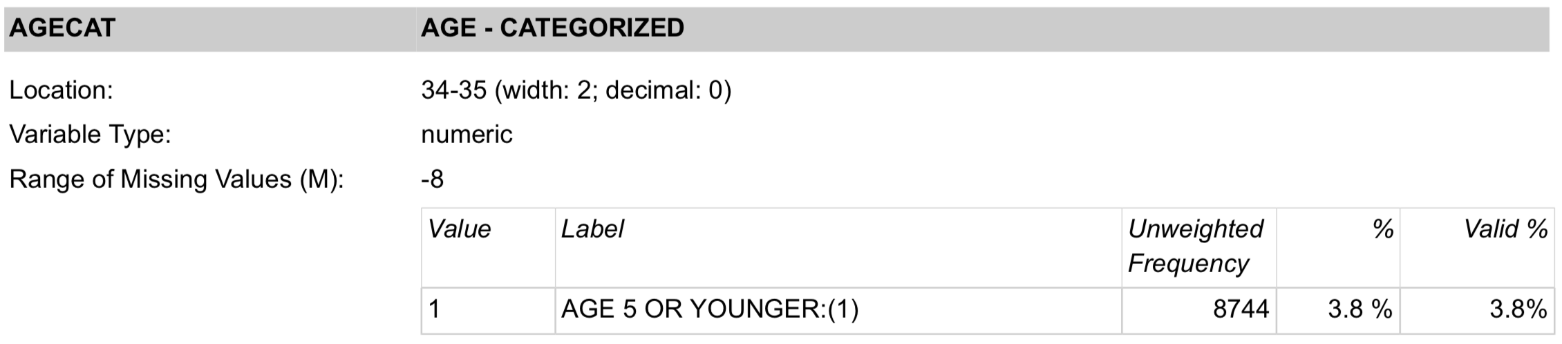
As noted earlier in this chapter, the DAWN file has fixed-width formatting, and we need to rely on a codebook to find out where the fields are. As an example, a snippet of the codebook in the figure below tells us that age appears in positions 34 and 35 in a row, and it is categorized into 11 age groups: 1 stands for age 5 and under, 2 for ages 6 to 11, ..., and 11 for ages 65 and older. Also,–8 represents a missing value.
 (Screenshot of a portion of the DAWN coding for age)
Earlier, we determined that the file contains 200,000 lines and over 280 million characters, so on average, there are about 1,200 characters per line. This might be why they used a fixed-width rather than a CSV format. Think how much larger the file would be if there was a comma between every field!
Given the tremendous amount of information on each line, let's read just a few features into a dataframe. We can use the pandas.read_fwf method to do this. We specify the exact positions of the fields to extract, and we provide names for these fields and other information about the header and index:
colspecs = [(0,6), (14,29), (33,35), (35, 37), (37, 39), (1213, 1214)]
varNames = ["id", "wt", "age", "sex", "race","type"]
dawn = pd.read_fwf('data/DAWN-Data.txt', colspecs=colspecs,
                   header=None, index_col=0, names=varNames)
dawn.head()
| wt | age | sex | race | type | |
|---|---|---|---|---|---|
| id | |||||
| 1 | 0.942635 | 4 | 1 | 2 | 8 |
| 2 | 5.992011 | 11 | 1 | 3 | 4 |
| 3 | 4.723172 | 11 | 2 | 2 | 4 |
| 4 | 4.080147 | 2 | 1 | 3 | 4 |
| 5 | 5.177709 | 6 | 1 | 3 | 8 |
We can compare the rows in the table to the number of lines in the file:
dawn.shape
(229211, 5)
The number of rows in the dataframe matches the number of lines in the file. That's good.
The granularity of the dataframe is a bit complicated due to the survey design. Recall that these data are part of a large scientific study, with a complex sampling scheme. A row represents an emergency room visit, so the granularity is at the emergency room visit level. However, in order to reflect the sampling scheme and be representative of the population of all drug-related ER visits in a year, weights are provided. We must apply the weight to each record when we compute summary statistics, build histograms, and fit models. (The wt field contains these values.)
The weights take into account the chance of an ER visit like this one appearing in the sample. By "like this one" we mean a visit with similar features, such as the visitor age, race, visit location, and time of day. Let's examine the different values in wt:
dawn['wt'].value_counts()
wt
0.938440     1719
84.258821    1617
1.724822     1435
1.135506     1278
4.921769     1274
             ...
6.038204        2
6.203833        1
1.511784        1
3.306254        1
3.330629        1
Name: count, Length: 3500, dtype: int64
Note: What do these weights mean? As a simplified example, suppose you ran a survey and 45% of your respondents were under 18 years of age, but according to the US Census Bureau, only 22% of the population is under 18. You can adjust your survey responses to reflect the US population by using a small weight (22/45) for those under 18 and a larger weight (78/55) for those 18 and older. To see how we might use these weights, suppose the respondents are asked whether they use Facebook:
| Facebook | < 18 | 18+ | Total
| :------------- | -------------: | -------------: |--------:
| No | 1 | 19 | 21
| Yes | 44 | 35 | 79
| Total | 45 | 55 | 100
Overall, 79% of the respondents say they are Facebook users, but the sample is skewed toward the younger generation. We can adjust the estimate with the weights so that the age groups match the population. Then the adjusted percentage of Facebook users drops to:
$$(22/45) \times 44 + (78/55) \times 35 = 71 $$
The DAWN survey uses the same idea, except that it splits the groups much more finely.
It is critical to include the survey weights in your analysis to get data that represents the population at large. For example, we can compare the calculation of the proportion of females among the ER visits both with and without the weights:
print(f'Unweighted percent female: {np.average(dawn["sex"] == 2):.1%}')
print(f'  Weighted percent female:',
      f'{np.average(dawn["sex"] == 2, weights=dawn["wt"]):.1%}')
Unweighted percent female: 48.0%
  Weighted percent female: 52.3%
These figures differ by more than 4 percentage points. The weighted version is a more accurate estimate of the proportion of females among the entire population of drug-related ER visits.
Sometimes the granularity can be tricky to figure out, like we saw with the inspections data. And at other times, we need to take sampling weights into account, like for the DAWN data. These examples show it's important to take your time and review the data descriptions before proceeding with analysis.
A.7 Summary
Data wrangling is an essential part of data analysis. Without it, we risk overlooking problems in data that can have major consequences for future analysis. This chapter covered an important first step in data wrangling: reading data from a plain-text source file into a Python dataframe and identifying its granularity. We introduced different types of file formats and encodings, and we wrote code that can read data from these formats. We checked the size of source files and considered alternative tools for working with large datasets.
We also introduced command-line tools as an alternative to Python for checking the format, encoding, and size of a file. These CLI tools are especially handy for filesystem-oriented tasks because of their simple syntax. We've only touched the surface of what CLI tools can do. In practice, the shell is capable of sophisticated data processing and is well worth learning.
Understanding the shape and granularity of a table gives us insight into what a row in a data table represents. This helps us determine whether the granularity is mixed, aggregation is needed, or weights are required. After looking at the granularity of your dataset, you should have answers to the following questions:
- What does a record represent? Clarity on this will help you correctly carry out a data analysis and state your findings.
- Do all records in a table capture granularity at the same level? Sometimes a table contains additional summary rows that have a different granularity, and you want to use only those rows that are at the right level of detail.
- If the data are aggregated, how was the aggregation performed? Summing and averaging are common types of aggregation. With averaged data, the variability in the measurements is typically reduced and relationships often appear stronger.
- What kinds of aggregations might you perform on the data? Aggregations might be useful or necessary to combine one data table with another.
Knowing your table’s granularity is a first step to cleaning your data, and it informs you of how to analyze the data. For example, we saw the granularity of the DAWN survey is an ER visit. That naturally leads us to think about comparisons of patient demographics to the US as a whole.
The wrangling techniques in this chapter help us bring data from a source file into a dataframe and understand its structure. Once we have a dataframe, further wrangling is needed to assess and improve quality and prepare the data for analysis. We cover these topics in the next chapter.