Lab-4 (SQL)

(Intro. to Data Science: IIT Delhi - Abu Dhabi)

Note: One of the agendas for this lab is to get started with relational databases. This is important as a data scientist since access to many datasets will be available through a database. We will also see SQL, the language for working with relational databases. This material is from Chapter 7 of [LDS].

In pandas, we used dataframes to represent tables of data. This chapter introduces relations, another widely used way to represent data tables. We also introduce SQL, the standard programming language for working with relations. Here's an example of a relation that holds information about popular dog breeds:

import pandas as pd
dogs = pd.read_csv('dogs.csv')

# Jupyter doesn't have a built-in way to display relations, so we jiggle the
# dataframe output a bit to make it look like a relation
from IPython.display import display, HTML
display(HTML(dogs.to_html(index=False)))

breed	grooming	food_cost	kids	size
Labrador Retriever	weekly	466.0	high	medium
German Shepherd	weekly	466.0	medium	large
Beagle	daily	324.0	high	small
Golden Retriever	weekly	466.0	high	medium
Yorkshire Terrier	daily	324.0	low	small
Bulldog	weekly	466.0	medium	medium
Boxer	weekly	466.0	high	medium

Like dataframes, each row in a relation represents a single record---in this case, a single dog breed. Each column represents a feature about the record---for example, the grooming column represents how often each dog breed needs to be groomed.

Both relations and dataframes have labels for each column in the table. However, one key difference is that the rows in a relation don't have labels, while rows in a dataframe do.

In this lab, we demonstrate common relation operations using SQL. We start by explaining the structure of SQL queries. Then we show how to use SQL to perform common data manipulation tasks, like slicing, filtering, sorting, grouping, and joining.

This chapter replicates the data analyses in Lab-2 using relations and SQL instead of dataframes and Python. The datasets, data manipulations, and conclusions are nearly identical across the two labs for ease of comparison between performing data manipulations in pandas and SQL.

1. Subsetting

To work with relations, we'll introduce a domain-specific programming language called SQL (Structured Query Language). We commonly pronounce "SQL" like "sequel" instead of spelling out the acronym. SQL is a specialized language for working with relations---as such, SQL has a different syntax than Python for writing programs that operate on relational data.

In this Lab, we'll use SQL queries within Python programs. This illustrates a common workflow---data scientists often process and subset data in SQL before loading the data into Python for further analysis. SQL databases make it easier to work with large amounts of data compared to pandas programs. However, loading data into pandas makes it easier to visualize the data and build statistical models.

Why do SQL systems tend to work better with larger datasets? In short, SQL systems have sophisticated algorithms for managing data stored on disk. For example, when working with a large dataset, SQL systems will transparently load and manipulate small portions of data at a time; doing this in pandas can be quite difficult in comparison. We cover this topic in more detail in a subsequent lab.

1.1 SQL Basics: SELECT and FROM

We'll use the pd.read_sql function, which runs a SQL query and stores the output in a pandas dataframe. Using this function requires some setup. We start by importing the pandas and sqlalchemy Python packages.

import pandas as pd
import sqlalchemy

Our database should be stored in a file called babynames.db. Please download it from here and store it in your working directory (i.e., the directory that has the Lab-4.ipynb file). This file is a SQLite database, so we'll set up a sqlalchemy object that can process this format:

db = sqlalchemy.create_engine('sqlite:///babynames.db')

In this book, we use SQLite, an extremely useful database system for working with data stored locally. Other systems make different trade-offs that are useful for different domains. For instance, PostgreSQL and MySQL are more complex systems that are useful for large web applications where many end users are writing data at the same time. Although each SQL system has slight differences, they provide the same core SQL functionality. Readers may also be aware that Python provides SQLite support in its standard sqlite3 library. We choose to use sqlalchemy because it's easier to reuse the code for other SQL systems beyond SQLite.

Now we can use pd.read_sql to run SQL queries on this database. This database has two relations: baby and nyt. Here's a simple example that reads in the entire baby relation:

# SQL query saved in a Python string
query = ''' 
SELECT *
FROM baby;
'''

pd.read_sql(query, db)

	Name	Sex	Count	Year
0	Liam	M	19659	2020
1	Noah	M	18252	2020
2	Oliver	M	14147	2020
3	Elijah	M	13034	2020
4	William	M	12541	2020
...	...	...	...	...
2020717	Ula	F	5	1880
2020718	Vannie	F	5	1880
2020719	Verona	F	5	1880
2020720	Vertie	F	5	1880
2020721	Wilma	F	5	1880

2020722 rows × 4 columns

The text inside the query variable contains SQL code. SELECT and FROM are SQL keywords. We read the preceding query like this:

SELECT *    -- Get all the columns...
FROM baby;  -- ...from the baby relation

The baby relation contains the same data as the baby dataframe in pandas: the names of all babies registered by the US Social Security Administration.

1.2 What's a Relation?

Let's examine the baby relation in more detail. A relation has rows and columns. Every column has a label, as illustrated below. Unlike dataframes, however, individual rows in a relation don't have labels. Also, unlike dataframes, rows of a relation aren't ordered.

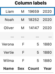
(The baby relation has labels for columns (boxed))

Relations have a long history. More formal treatments of relations use the term tuple to refer to the rows of a relation, and attribute to refer to the columns. There is also a rigorous way to define data operations using relational algebra, which is derived from mathematical set algebra.

1.3 Slicing

Slicing is an operation that creates a new relation by taking a subset of rows or columns out of another relation. Think about slicing a tomato---slices can go both vertically and horizontally. To slice columns of a relation, we give the SELECT statement the columns we want:

query = ''' 
SELECT Name
FROM baby;
''' 

pd.read_sql(query, db)

query = ''' 
SELECT Name, Count
FROM baby;
''' 

pd.read_sql(query, db)

To slice out a specific number of rows, use the LIMIT keyword:

query = ''' 
SELECT Name
FROM baby
LIMIT 10;
''' 

pd.read_sql(query, db)

In summary, we use the SELECT and LIMIT keywords to slice columns and rows of a relation.

1.4 Filtering Rows

Now we turn to filtering rows---taking subsets of rows using one or more criteria. In pandas, we slice dataframes using Boolean series objects. In SQL, we instead use the WHERE keyword with a predicate. The following query filters the baby relation to have only the baby names in 2020:

query = ''' 
SELECT *
FROM baby
WHERE Year = 2020;
'''

pd.read_sql(query, db)

	Name	Sex	Count	Year
0	Liam	M	19659	2020
1	Noah	M	18252	2020
2	Oliver	M	14147	2020
3	Elijah	M	13034	2020
4	William	M	12541	2020
...	...	...	...	...
31265	Zykeria	F	5	2020
31266	Zylani	F	5	2020
31267	Zylynn	F	5	2020
31268	Zynique	F	5	2020
31269	Zynlee	F	5	2020

31270 rows × 4 columns

Warning: Note that when comparing for equality, SQL uses a single equals sign:

SELECT *
FROM baby
WHERE Year = 2020;
--         ↑
--         Single equals sign

In Python, however, single equals signs are used for variable assignment. The statement Year = 2020 will assign the value 2020 to the variable Year. To compare for equality, Python code uses double equals signs:

# Assignment
my_year = 2021

# Comparison, which evaluates to False
my_year == 2020

To add more predicates to the filter, use the AND and OR keywords. For instance, to find the names that have more than 10,000 babies in either 2020 or 2019, we write:

query = ''' 
SELECT *
FROM baby
WHERE Count > 10000
  AND (Year = 2020
       OR Year = 2019);
-- Notice that we use parentheses to enforce evaluation order
'''

pd.read_sql(query, db)

	Name	Sex	Count	Year
0	Liam	M	19659	2020
1	Noah	M	18252	2020
2	Oliver	M	14147	2020
3	Elijah	M	13034	2020
4	William	M	12541	2020
5	James	M	12250	2020
6	Benjamin	M	12136	2020
7	Lucas	M	11281	2020
8	Henry	M	10705	2020
9	Alexander	M	10151	2020
10	Mason	M	10029	2020
11	Emma	F	15581	2020
12	Ava	F	13084	2020
13	Charlotte	F	13003	2020
14	Sophia	F	12976	2020
15	Amelia	F	12704	2020
16	Isabella	F	12066	2020
17	Mia	F	11157	2020
18	Liam	M	20555	2019
19	Noah	M	19097	2019
20	Oliver	M	13929	2019
21	William	M	13599	2019
22	Elijah	M	13339	2019
23	James	M	13131	2019
24	Benjamin	M	12980	2019
25	Lucas	M	12445	2019
26	Mason	M	11436	2019
27	Ethan	M	11265	2019
28	Alexander	M	11264	2019
29	Henry	M	10737	2019
30	Jacob	M	10721	2019
31	Michael	M	10558	2019
32	Daniel	M	10531	2019
33	Logan	M	10520	2019
34	Jackson	M	10128	2019
35	Emma	F	17155	2019
36	Ava	F	14474	2019
37	Sophia	F	13753	2019
38	Isabella	F	13344	2019
39	Charlotte	F	13191	2019
40	Amelia	F	12900	2019
41	Mia	F	12452	2019
42	Harper	F	10464	2019
43	Evelyn	F	10412	2019

Finally, to find the 10 most common names in 2020, we can sort the dataframe by Count in descending order using the ORDER BY keyword with the DESC option (short for DESCending):

query = ''' 
SELECT *
FROM baby
WHERE Year = 2020
ORDER BY Count DESC
LIMIT 10;
'''

pd.read_sql(query, db)

	Name	Sex	Count	Year
0	Liam	M	19659	2020
1	Noah	M	18252	2020
2	Emma	F	15581	2020
3	Oliver	M	14147	2020
4	Ava	F	13084	2020
5	Elijah	M	13034	2020
6	Charlotte	F	13003	2020
7	Sophia	F	12976	2020
8	Amelia	F	12704	2020
9	William	M	12541	2020

We see that Liam, Noah, and Emma were the most popular baby names in 2020.

1.5 Example: How Recently Has Luna Become a Popular Name?

As we mentioned in Lab-2, a New York Times article mentions that the name Luna was almost nonexistent before 2000 but has since grown to become a very popular name for girls. When exactly did Luna become popular? We can check this in SQL using slicing and filtering:

query = ''' 
SELECT *
FROM baby
WHERE Name = "Luna"
  AND Sex = "F";
'''

luna = pd.read_sql(query, db)
luna

	Name	Sex	Count	Year
0	Luna	F	7770	2020
1	Luna	F	7772	2019
2	Luna	F	6929	2018
3	Luna	F	5351	2017
4	Luna	F	3677	2016
...	...	...	...	...
123	Luna	F	15	1885
124	Luna	F	18	1884
125	Luna	F	17	1883
126	Luna	F	18	1881
127	Luna	F	15	1880

128 rows × 4 columns

pd.read_sql returns a pandas.DataFrame object, which we can use to make a plot. This illustrates a common workflow—process the data using SQL, load it into a pandas dataframe, then visualize the results:

from matplotlib.pyplot import subplots

fig, ax = subplots(figsize = (4, 4))
ax.plot(luna['Year'], luna['Count']);

In this section, we introduced the common ways that data scientists subset relations---slicing with column labels and filtering using a boolean condition. In the next section, we explain how to aggregate rows together.

2. Aggregating

his section introduces grouping and aggregating in SQL. We'll work with the baby names data, as in the previous section:

query = ''' 
SELECT *
FROM baby
LIMIT 10
'''

pd.read_sql(query, db)

	Name	Sex	Count	Year
0	Liam	M	19659	2020
1	Noah	M	18252	2020
2	Oliver	M	14147	2020
3	Elijah	M	13034	2020
4	William	M	12541	2020
5	James	M	12250	2020
6	Benjamin	M	12136	2020
7	Lucas	M	11281	2020
8	Henry	M	10705	2020
9	Alexander	M	10151	2020

2.1 Basic Group-Aggregate Using GROUP BY

Let's say we want to find out the total number of babies born as recorded in this data. This is simply the sum of the Count column. SQL provides functions that we use in the SELECT statement, like SUM:

query = '''
SELECT SUM(Count)
FROM baby
'''

pd.read_sql(query, db)

	SUM(Count)
0	352554503

In Lab-2, we used grouping and aggregation to figure out whether US births are trending upward over time. We grouped the dataset by year using .groupby(), then summed the counts within each group using .sum().

In SQL, we instead group using the GROUP BY clause, then call aggregation functions in SELECT:

query = ''' 
SELECT Year, SUM(Count)
FROM baby
GROUP BY Year
'''

pd.read_sql(query, db)

	Year	SUM(Count)
0	1880	194419
1	1881	185772
2	1882	213385
3	1883	208932
4	1884	234244
...	...	...
136	2016	3642755
137	2017	3548457
138	2018	3487193
139	2019	3437438
140	2020	3287724

141 rows × 2 columns

As with dataframe grouping, notice that the Year column contains the unique Year values---there are no duplicate Year values anymore since we grouped them together. When grouping in pandas, the grouping columns become the index of the resulting dataframe. However, relations don't have row labels, so the Year values are just a column in the resulting relation.

Here's the basic recipe for grouping in SQL:

SELECT
  col1,           -- column used for grouping
  SUM(col2)       -- aggregation of another column
FROM table_name   -- relation to use
GROUP BY col1     -- the column(s) to group by

Note that the order of clauses in a SQL statement is important. To avoid a syntax error, SELECT needs to appear first, then FROM, then WHERE, then GROUP BY.

When using GROUP BY we need to be careful about the columns given to SELECT. In general, we can only include columns without an aggregation when we use those columns to group. For instance, in the preceding example we grouped by the Year column, so we can include Year in the SELECT clause. All other columns included in SELECT should be aggregated, as we did earlier with SUM(Count). If we included a "bare" column like Name that wasn't used for grouping, it's ambiguous which name within the group should be returned. Although bare columns won't cause an error for SQLite, they cause other SQL engines to error, so we recommend avoiding them.

2.2 Grouping on Multiple Columns

We pass multiple columns into GROUP BY to group by multiple columns at once. This is useful when we need to further subdivide our groups. For example, we can group by both year and sex to see how many male and female babies were born over time:

query = ''' 
SELECT Year, Sex, SUM(Count)
FROM baby
GROUP BY Year, Sex
'''

pd.read_sql(query, db)

	Year	Sex	SUM(Count)
0	1880	F	83929
1	1880	M	110490
2	1881	F	85034
3	1881	M	100738
4	1882	F	99699
...	...	...	...
277	2018	M	1810309
278	2019	F	1651911
279	2019	M	1785527
280	2020	F	1581301
281	2020	M	1706423

282 rows × 3 columns

Notice that the preceding code is very similar to grouping by a single column, except that it gives multiple columns to GROUP BY to group by both Year and Sex.

Note: Unlike `pandas`, SQLite doesn't provide a simple way to pivot a relation. Instead, we can use `GROUP BY` on two columns in SQL, read the result into a dataframe, and then use the `unstack()` dataframe method.

2.3 Other Aggregation Functions

SQLite has several other built-in aggregation functions besides SUM, such as COUNT, AVG, MIN, and MAX. For the full list of functions, consult the SQLite website.

To use another aggregation function, we call it in the SELECT clause. For instance, we can use MAX instead of SUM:

query = ''' 
SELECT Year, MAX(Count)
FROM baby
GROUP BY Year
'''

pd.read_sql(query, db)

	Year	MAX(Count)
0	1880	9655
1	1881	8769
2	1882	9557
3	1883	8894
4	1884	9388
...	...	...
136	2016	19380
137	2017	18824
138	2018	19924
139	2019	20555
140	2020	19659

141 rows × 2 columns

The built-in aggregation functions are one of the first places a data scientist may encounter differences in SQL implementations. For instance, SQLite has a relatively minimal set of aggregation functions while PostgreSQL has many more. That said, almost all SQL implementations provide SUM, COUNT, MIN, MAX, and AVG.

This section covered common ways to aggregate data in SQL using the GROUP BY keyword with one or more columns. In the next section, we'll explain how to join relations together.

3. Joining

To connect records between two data tables, SQL relations can be joined together similar to dataframes. In this section, we introduce SQL joins to replicate our analysis of the baby names data. Recall that Lab-2 mentions a New York Times article that talks about how certain name categories, like mythological and baby boomer names, have become more or less popular over time.

We've taken the names and categories in the NYT article and put them in a small relation named nyt:

query = ''' 
SELECT *
FROM nyt;
'''

pd.read_sql(query, db)

	nyt_name	category
0	Lucifer	forbidden
1	Lilith	forbidden
2	Danger	forbidden
3	Amen	evangelical
4	Savior	evangelical
5	Canaan	evangelical
6	Creed	evangelical
7	Saint	evangelical
8	Susan	boomer
9	Debbie	boomer
10	Bobby	boomer
11	Karen	boomer
12	Julius	mythology
13	Cassius	mythology
14	Freya	mythology
15	Hera	mythology
16	Nyx	mythology
17	Osiris	mythology
18	Onyx	mineral
19	Amethyst	mineral
20	Venus	celestial
21	Celestia	celestial
22	Skye	celestial

Note: Notice that the preceding code runs a query on `babynames.db`, the same database that contains the larger `baby` relation from the previous sections. SQL databases can hold more than one relation, making them very useful when we need to work with many data tables at once. CSV files, on the other hand, typically contain one data table each---if we perform a data analysis that uses 20 data tables, we might need to keep track of the names, locations, and versions of 20 CSV files. Instead, it could be simpler to store all the data tables in a SQLite database stored in a single file.

To see how popular the categories of names are, we join the nyt relation with the baby relation to get the name counts from baby.

3.1 Inner Joins

As in Lab-2, we've made smaller versions of the baby and nyt tables so that it's easier to see what happens when we join tables together. The relations are called baby_small and nyt_small:

query = ''' 
SELECT *
FROM baby_small;
'''

pd.read_sql(query, db)

	Name	Sex	Count	Year
0	Noah	M	18252	2020
1	Julius	M	960	2020
2	Karen	M	6	2020
3	Karen	F	325	2020
4	Noah	F	305	2020

query = ''' 
SELECT *
FROM nyt_small;
'''

pd.read_sql(query, db)

	nyt_name	category
0	Karen	boomer
1	Julius	mythology
2	Freya	mythology

To join relations in SQL, we use the INNER JOIN clause to say which tables we want to join and the ON clause to specify a predicate for joining the tables. Here's an example:

query = ''' 
SELECT *
FROM baby_small INNER JOIN nyt_small
  ON baby_small.Name = nyt_small.nyt_name
'''

pd.read_sql(query, db)

	Name	Sex	Count	Year	nyt_name	category
0	Julius	M	960	2020	Julius	mythology
1	Karen	M	6	2020	Karen	boomer
2	Karen	F	325	2020	Karen	boomer

Notice that this result is the same as doing an inner join in pandas: the new table has the columns of both the baby_small and nyt_small tables. The rows with the name Noah are gone, and the remaining rows have their matching category from nyt_small.

To join two tables together, we tell SQL the column(s) from each table that we want to use to do the join using a predicate with the ON keyword. SQL matches rows together when the values in the joining columns fulfill the predicate, as shown in the figure below.

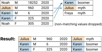
(Joining two tables together with SQL)

Unlike pandas, SQL gives more flexibility on how rows are joined. The pd.merge() method can only join using simple equality, but the predicate in the ON clause can be arbitrarily complex. As an example, we take advantage of this extra versatility in later labs.

3.2 Left and Right Joins

Like pandas, SQL also supports left joins. Instead of saying INNER JOIN, we use LEFT JOIN:

query = ''' 
SELECT *
FROM baby_small LEFT JOIN nyt_small
  ON baby_small.Name = nyt_small.nyt_name
'''

pd.read_sql(query, db)

	Name	Sex	Count	Year	nyt_name	category
0	Noah	M	18252	2020	None	None
1	Julius	M	960	2020	Julius	mythology
2	Karen	M	6	2020	Karen	boomer
3	Karen	F	325	2020	Karen	boomer
4	Noah	F	305	2020	None	None

As we might expect, the "left" side of the join refers to the table that appears on the left side of the LEFT JOIN keyword. We can see the Noah rows are kept in the resulting relation even when they don't have a match in the righthand relation.

Note that SQLite doesn't support right joins directly, but we can perform the same join by swapping the order of relations, then using LEFT JOIN:

query = ''' 
SELECT *
FROM nyt_small LEFT JOIN baby_small
  ON baby_small.Name = nyt_small.nyt_name
'''

pd.read_sql(query, db)

	nyt_name	category	Name	Sex	Count	Year
0	Karen	boomer	Karen	F	325.0	2020.0
1	Karen	boomer	Karen	M	6.0	2020.0
2	Julius	mythology	Julius	M	960.0	2020.0
3	Freya	mythology	None	None	NaN	NaN

SQLite doesn't have a built-in keyword for outer joins. In cases where an outer join is needed, we have to either use a different SQL engine or perform an outer join via pandas. However, in our (the authors') experience, outer joins are rarely used in practice compared to inner and left joins.

3.3 Example: Popularity of NYT Name Categories

Now let's return to the full baby and nyt relations.

We want to know how the popularity of name categories in nyt has changed over time. To answer this question, we should:

1. Inner join baby with nyt, matching rows where the names are equal.
2. Group the table by category and Year.
3. Aggregate the counts using a sum:

query = ''' 
SELECT
  category,
  Year,
  SUM(Count) AS count           -- [3]
FROM baby INNER JOIN nyt        -- [1]
  ON baby.Name = nyt.nyt_name   -- [1]
GROUP BY category, Year         -- [2]
'''

cate_counts = pd.read_sql(query, db)
cate_counts

	category	Year	count
0	boomer	1880	292
1	boomer	1881	298
2	boomer	1882	326
3	boomer	1883	322
4	boomer	1884	335
...	...	...	...
645	mythology	2016	2671
646	mythology	2017	2797
647	mythology	2018	2944
648	mythology	2019	3320
649	mythology	2020	3489

650 rows × 3 columns

The numbers in square brackets ([1], [2], [3]) in the preceding query show how each step in our plan maps to the parts of the SQL query. The code re-creates the dataframe from Lab-2, where we created plots to verify the claims of the New York Times article. For brevity, we omit duplicating the plots here.

Note: Notice that in the SQL code in this example, the numbers appear out of order---[3], [1], then [2]. As a rule of thumb for first-time SQL learners, we can often think of the SELECT statement as the last piece of the query to execute even though it appears first.

In this section, we introduced joins for relations. When joining relations together, we match rows using the INNER JOIN or LEFT JOIN keyword and a boolean predicate. In the next section, we'll explain how to transform values in a relation.

4. Transforming and Common Table Expressions

In this section, we show how to call functions to transform columns of data using built-in SQL functions. We also demonstrate how to use common table expressions to build up complex queries from simpler ones. As usual, we start by loading the database:

# Set up connection to database
import sqlalchemy
db = sqlalchemy.create_engine('sqlite:///babynames.db')

4.1 SQL Functions

SQLite provides a variety of scalar functions, or functions that transform single data values. When called on a column of data, SQLite will apply these functions on each value in the column. In contrast, aggregation functions like SUM and COUNT take a column of values as input and compute a single value as output.

SQLite provides a comprehensive list of the built-in scalar functions in its online documentation. For instance, to find the number of characters in each name, we use the LENGTH function:

query = ''' 
SELECT Name, LENGTH(Name)
FROM baby
LIMIT 10;
'''

pd.read_sql(query, db)

	Name	LENGTH(Name)
0	Liam	4
1	Noah	4
2	Oliver	6
3	Elijah	6
4	William	7
5	James	5
6	Benjamin	8
7	Lucas	5
8	Henry	5
9	Alexander	9

Notice that the LENGTH function is applied to each value within the Name column.

Note: Like aggregation functions, each implementation of SQL provides a different set of scalar functions. SQLite has a relatively minimal set of functions, while PostgreSQL has many more. That said, almost all SQL implementations provide some equivalent to SQLite's LENGTH, ROUND, SUBSTR, and LIKE functions.

Although scalar functions use the same syntax as an aggregation function, they behave differently. This can result in confusing output if the two are mixed together in a single query:

query = ''' 
SELECT Name, LENGTH(Name), AVG(Count)
FROM baby
LIMIT 10;
'''

pd.read_sql(query, db)

	Name	LENGTH(Name)	AVG(Count)
0	Liam	4	174.469572

Here, the AVG(Name) computes the average of the entire Count column, but the output is confusing---a reader could easily think the average is related to the name Liam. For this reason, we must be careful when scalar and aggregation functions appear together within a SELECT statement.

To extract the first letter of each name, we can use the SUBSTR function (short for substring). As described in the documentation, the SUBSTR function takes three arguments. The first is the input string, the second is the position to begin the substring (1-indexed), and the third is the length of the substring:

query = ''' 
SELECT Name, SUBSTR(Name, 1, 1)
FROM baby
LIMIT 10;
'''

pd.read_sql(query, db)

	Name	SUBSTR(Name, 1, 1)
0	Liam	L
1	Noah	N
2	Oliver	O
3	Elijah	E
4	William	W
5	James	J
6	Benjamin	B
7	Lucas	L
8	Henry	H
9	Alexander	A

We can use the AS keyword to rename the column:

query = ''' 
SELECT *, SUBSTR(Name, 1, 1) AS Firsts
FROM baby
LIMIT 10;
'''

pd.read_sql(query, db)

	Name	Sex	Count	Year	Firsts
0	Liam	M	19659	2020	L
1	Noah	M	18252	2020	N
2	Oliver	M	14147	2020	O
3	Elijah	M	13034	2020	E
4	William	M	12541	2020	W
5	James	M	12250	2020	J
6	Benjamin	M	12136	2020	B
7	Lucas	M	11281	2020	L
8	Henry	M	10705	2020	H
9	Alexander	M	10151	2020	A

After calculating the first letter of each name, our analysis aims to understand the popularity of first letters over time. To do this, we want to take the output of this SQL query and use it as a single step within a longer chain of operations.

SQL provides several options to break queries into smaller steps, which is helpful in more complex analyses like this one. The most common options for doing this are to create a new relation using a CREATE TABLE statement, create a new view using CREATE VIEW, or create a temporary relation using WITH. Each of these methods have different use-cases. For simplicity, we only describe the WITH statement in this section and suggest that readers look over the SQLite documentation for details.

4.2 Multistep Queries Using a WITH Clause

The WITH clause lets us assign a name to any SELECT query. Then we can treat that query as though it exists as a relation in the database just for the duration of the query. SQLite calls these temporary relations common table expressions. For instance, we can take the earlier query that calculates the first letter of each name and call it letters:

query = ''' 
-- Create a temporary relation called letters by calculating
-- the first letter for each name in baby
WITH letters AS (
  SELECT *, SUBSTR(Name, 1, 1) AS Firsts
  FROM baby
)
-- Then, select the first ten rows from letters
SELECT *
FROM letters
LIMIT 10;
'''

pd.read_sql(query, db)

	Name	Sex	Count	Year	Firsts
0	Liam	M	19659	2020	L
1	Noah	M	18252	2020	N
2	Oliver	M	14147	2020	O
3	Elijah	M	13034	2020	E
4	William	M	12541	2020	W
5	James	M	12250	2020	J
6	Benjamin	M	12136	2020	B
7	Lucas	M	11281	2020	L
8	Henry	M	10705	2020	H
9	Alexander	M	10151	2020	A

WITH statements are very useful since they can be chained together. We can create multiple temporary relations in a WITH statement that each perform a bit of work on the previous result, which lets us gradually build complicated queries a step at a time.

4.3 Example: Popularity of "L" Names

We can use WITH statements to look at the popularity of names that start with the letter L over time. We'll group the temporary letters relation by the first letter and year, then aggregate the Count column using a sum, then filter to get only names with the letter L:

query = ''' 
WITH letters AS (
  SELECT *, SUBSTR(Name, 1, 1) AS Firsts
  FROM baby
)
SELECT Firsts, Year, SUM(Count) AS Count
FROM letters
WHERE Firsts = "L"
GROUP BY Firsts, Year;
'''

letter_counts = pd.read_sql(query, db)
letter_counts

	Firsts	Year	Count
0	L	1880	12799
1	L	1881	12770
2	L	1882	14923
3	L	1883	15106
4	L	1884	16742
...	...	...	...
136	L	2016	243440
137	L	2017	247243
138	L	2018	246251
139	L	2019	249315
140	L	2020	239760

141 rows × 3 columns

This relation contains the same data as the one from Lab-2. In that Lab, we made a plot of the Count column over time, which we omit here for brevity.

In this section, we introduced data transformations. To transform values in a relation, we commonly use SQL functions like LENGTH() or SUBSTR(). We also explained how to build up complex queries using the WITH clause.

5. Summary

Here, we explained what relations are, why they're useful, and how to work with them using SQL code. SQL databases are useful for many real-world settings. For example, SQL databases typically have robust data recovery mechanisms---if the computer crashes while in the middle of a SQL operation, the database system can recover as much data as possible without corruption. As mentioned earlier, SQL databases can also handle larger scale; organizations use SQL databases to store and query databases that are far too large to analyze in-memory using pandas code. These are just a few reasons why SQL is an important part of the data science toolbox, and we expect that many readers will soon encounter SQL code as part of their work.