(Lab 2). Working with Dataframes Using pandas
Data scientists work with data stored in tables. This chapter introduces
dataframes, one of the most widely used ways to represent data tables. We
also introduce pandas, the standard Python package for working with
dataframes. Here is an example of a dataframe that holds information about
popular dog breeds:
import pandas as pd
dogs = pd.read_csv('all_dogs.csv', index_col='breed')

dogs
| group | datadog | popularity_all | popularity | lifetime_cost | intelligence_rank | longevity | ailments | price | food_cost | grooming | kids | megarank_kids | megarank | size | weight | height | |
|---|---|---|---|---|---|---|---|---|---|---|---|---|---|---|---|---|---|
| breed | |||||||||||||||||
| Border Collie | herding | 3.64 | 45 | 39.0 | 20143.0 | 1.0 | 12.52 | 2.0 | 623.0 | 324.0 | weekly | low | 1.0 | 29.0 | medium | NaN | 20.0 |
| Border Terrier | terrier | 3.61 | 80 | 61.0 | 22638.0 | 30.0 | 14.00 | 0.0 | 833.0 | 324.0 | weekly | high | 2.0 | 1.0 | small | 13.5 | NaN |
| Brittany | sporting | 3.54 | 30 | 30.0 | 22589.0 | 19.0 | 12.92 | 0.0 | 618.0 | 466.0 | weekly | medium | 3.0 | 11.0 | medium | 35.0 | 19.0 |
| Cairn Terrier | terrier | 3.53 | 59 | 48.0 | 21992.0 | 35.0 | 13.84 | 2.0 | 435.0 | 324.0 | weekly | high | 4.0 | 2.0 | small | 14.0 | 10.0 |
| Welsh Springer Spaniel | sporting | 3.34 | 130 | 81.0 | 20224.0 | 31.0 | 12.49 | 1.0 | 750.0 | 324.0 | weekly | high | 5.0 | 4.0 | medium | NaN | 18.0 |
| ... | ... | ... | ... | ... | ... | ... | ... | ... | ... | ... | ... | ... | ... | ... | ... | ... | ... |
| Weimaraner | sporting | NaN | 32 | NaN | NaN | 21.0 | NaN | 1.0 | 562.0 | NaN | weekly | high | NaN | NaN | large | NaN | 25.0 |
| Welsh Terrier | terrier | NaN | 99 | NaN | NaN | 53.0 | NaN | 0.0 | 843.0 | NaN | weekly | high | NaN | NaN | small | 20.0 | 15.0 |
| Wire Fox Terrier | terrier | NaN | 100 | NaN | NaN | 51.0 | 13.17 | 0.0 | 668.0 | NaN | NaN | NaN | NaN | NaN | small | 17.5 | 15.0 |
| Wirehaired Pointing Griffon | sporting | NaN | 92 | NaN | NaN | 46.0 | 8.80 | 0.0 | 755.0 | NaN | NaN | NaN | NaN | NaN | medium | NaN | 22.0 |
| Xoloitzcuintli | non-sporting | NaN | 155 | NaN | NaN | NaN | NaN | NaN | 717.0 | NaN | NaN | NaN | NaN | NaN | medium | NaN | 16.5 |
172 rows × 17 columns
In a dataframe, each row represents a single record---in this case, a single dog breed. Each column represents a feature about the record---for example, the grooming column represents how often each dog breed needs to be groomed.
Dataframes have labels for both columns and rows. For instance, this dataframe has a column labeled grooming and a row labeled German Shepherd. The columns and rows of a dataframe are ordered—we can refer to the Labrador Retriever row as the first row of the dataframe.
Within a column, data have the same type. For instance, the the cost of food contains numbers, and the size of the dog consists of categories. But data types can be different within a row.
Because of these properties, dataframes enable all sorts of useful operations.
Other times, people use the same term to refer to slightly different ideas. Data types in a programming sense refers to how a computer stores data internally. For instance, the size column has a string data type in Python. But from a statistical point of view, the type of the size column is ordered categorical data (ordinal data).
In this Lab, we introduce common dataframe operations using
pandas. Data scientists use the pandas library when working with dataframes
in Python. First, we explain the main objects that pandas provides: the
DataFrame and Series classes. Then we show how to use pandas to
perform common data manipulation tasks, like slicing, filtering, sorting,
grouping, and joining.
2.1 Subsetting
This section introduces operations for taking subsets of dataframes. When data scientists first read in a dataframe, they often want to subset the specific data that they plan to use. For example, a data scientist can slice out the 10 relevant features from a dataframe with hundreds of columns. Or they can filter a dataframe to remove rows with incomplete data. For the rest of this lab, we demonstrate dataframe operations using a dataframe of baby names.
Data Scope and Question
There's a 2021 New York Times article that talks about Prince Harry and
Meghan Markle's unique choice for their new baby daughter's name: Lilibet. The article has an interview with Pamela Redmond,
an expert on baby names, who talks about interesting trends in how people name
their kids. For example, she says that names that start with the letter L
have become very popular in recent years, while names that start with the
letter J were most popular in the 1970s and 1980s. Are these claims reflected
in data? We can use pandas to find out.
First, we import the package as pd, the canonical abbreviation:
import pandas as pd
We have a dataset of baby names stored in a comma-separated values (CSV) file
called babynames.csv. We use the pd.read_csv function to read the file as a
pandas.DataFrame object:
baby = pd.read_csv('babynames.csv')
baby
| Name | Sex | Count | Year | |
|---|---|---|---|---|
| 0 | Liam | M | 19659 | 2020 |
| 1 | Noah | M | 18252 | 2020 |
| 2 | Oliver | M | 14147 | 2020 |
| 3 | Elijah | M | 13034 | 2020 |
| 4 | William | M | 12541 | 2020 |
| ... | ... | ... | ... | ... |
| 2020717 | Ula | F | 5 | 1880 |
| 2020718 | Vannie | F | 5 | 1880 |
| 2020719 | Verona | F | 5 | 1880 |
| 2020720 | Vertie | F | 5 | 1880 |
| 2020721 | Wilma | F | 5 | 1880 |
2020722 rows × 4 columns
The data in the baby table comes from the US Social Security Administration (SSA),
which records the baby name and birth sex for birth certificate purposes. The SSA makes the baby names data available on its website.
We've loaded this data into the baby table.
The SSA website has a page that describes the data in more detail. We won't go in depth in this chapter about the data's limitations, but we'll point out this relevant information from the website:
All names are from Social Security card applications for births that occurred in the United States after 1879. Note that many people born before 1937 never applied for a Social Security card, so their names are not included in our data. For others who did apply, our records may not show the place of birth, and again their names are not included in our data.
All data are from a 100% sample of our records on Social Security card applications as of March 2021.
It's also important to point out that at the time of this writing, the SSA dataset only provides the binary options of male and female. We hope that in the future, national datasets like this one will provide more inclusive options.
Dataframes and Indices
Let's examine the baby dataframe in more detail. A dataframe has rows and
columns. Every row and column has a label, as highlighted in the figure below:
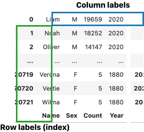
(The baby dataframe has labels for both rows and columns (boxed))
By default, pandas assigns row labels as incrementing numbers starting from
0. In this case, the data at the row labeled 0 and column labeled Name has
the data 'Liam'.
Dataframes can also have strings as row labels. The figure below shows a dataframe of dog data where the row labels are strings.
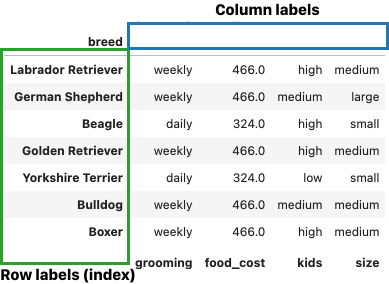
(Row labels in dataframes can also be strings, as in this example, in which each row is labeled using the dog breed name)
The row labels have a special name. We call them the index of a dataframe,
and pandas stores the row labels in a special pd.Index object. We won't
discuss the pd.Index object since it's less common to manipulate the
index itself. For now, it's important to remember that even though the index looks
like a column of data, the index really represents row labels, not data. For
instance, the dataframe of dog breeds has four columns of data, not five, since
the index doesn't count as a column.
Slicing
Slicing is an operation that creates a new dataframe by taking a subset of
rows or columns out of another dataframe. Think about slicing a tomato---slices
can go both vertically and horizontally. To take slices of a dataframe in
pandas, we use the .loc and .iloc properties. Let's start with .loc.
Here's the full baby dataframe:
baby
| Name | Sex | Count | Year | |
|---|---|---|---|---|
| 0 | Liam | M | 19659 | 2020 |
| 1 | Noah | M | 18252 | 2020 |
| 2 | Oliver | M | 14147 | 2020 |
| 3 | Elijah | M | 13034 | 2020 |
| 4 | William | M | 12541 | 2020 |
| ... | ... | ... | ... | ... |
| 2020717 | Ula | F | 5 | 1880 |
| 2020718 | Vannie | F | 5 | 1880 |
| 2020719 | Verona | F | 5 | 1880 |
| 2020720 | Vertie | F | 5 | 1880 |
| 2020721 | Wilma | F | 5 | 1880 |
2020722 rows × 4 columns
.loc lets us select rows and columns using their labels. For example, to get the data in the row labeled 1 and column labeled Name:
#        The first argument is the row label
#        ↓
baby.loc[1, 'Name']
#            ↑
#            The second argument is the column label
'Noah'
To slice out multiple rows or columns, we can use Python slice syntax instead of individual values:
baby.loc[0:3, 'Name':'Count']
| Name | Sex | Count | |
|---|---|---|---|
| 0 | Liam | M | 19659 |
| 1 | Noah | M | 18252 |
| 2 | Oliver | M | 14147 |
| 3 | Elijah | M | 13034 |
To get an entire column of data, we can pass an empty slice as the first argument:
baby.loc[:, 'Count']
0          19659
1          18252
2          14147
3          13034
4          12541
           ...
2020717        5
2020718        5
2020719        5
2020720        5
2020721        5
Name: Count, Length: 2020722, dtype: int64
Notice that the output of this doesn't look like a dataframe, and it's not.
Selecting out a single row or column of a dataframe produces a pd.Series
object:
counts = baby.loc[:, 'Count']
counts.__class__.__name__
'Series'
What's the difference between a pd.Series object and a pd.DataFrame object?
Essentially, a pd.DataFrame is two-dimensional---it has rows and columns and
represents a table of data. A pd.Series is one-dimensional---it represents a
list of data. pd.Series and pd.DataFrame objects have many methods in
common, but they really represent two different things. Confusing the two can
cause bugs and confusion.
To select specific columns of a dataframe, pass a list into .loc:
# Here's the original dataframe
baby
| Name | Sex | Count | Year | |
|---|---|---|---|---|
| 0 | Liam | M | 19659 | 2020 |
| 1 | Noah | M | 18252 | 2020 |
| 2 | Oliver | M | 14147 | 2020 |
| 3 | Elijah | M | 13034 | 2020 |
| 4 | William | M | 12541 | 2020 |
| ... | ... | ... | ... | ... |
| 2020717 | Ula | F | 5 | 1880 |
| 2020718 | Vannie | F | 5 | 1880 |
| 2020719 | Verona | F | 5 | 1880 |
| 2020720 | Vertie | F | 5 | 1880 |
| 2020721 | Wilma | F | 5 | 1880 |
2020722 rows × 4 columns
# And here's the dataframe with only Name and Year columns
baby.loc[:, ['Name', 'Year']]
#           └──────┬───────┘
#         list of column labels
| Name | Year | |
|---|---|---|
| 0 | Liam | 2020 |
| 1 | Noah | 2020 |
| 2 | Oliver | 2020 |
| 3 | Elijah | 2020 |
| 4 | William | 2020 |
| ... | ... | ... |
| 2020717 | Ula | 1880 |
| 2020718 | Vannie | 1880 |
| 2020719 | Verona | 1880 |
| 2020720 | Vertie | 1880 |
| 2020721 | Wilma | 1880 |
2020722 rows × 2 columns
Selecting columns is very common, so there's a shorthand:
# Shorthand for baby.loc[:, ['Name', 'Count']]
baby[['Name', 'Count']]
| Name | Count | |
|---|---|---|
| 0 | Liam | 19659 |
| 1 | Noah | 18252 |
| 2 | Oliver | 14147 |
| 3 | Elijah | 13034 |
| 4 | William | 12541 |
| ... | ... | ... |
| 2020717 | Ula | 5 |
| 2020718 | Vannie | 5 |
| 2020719 | Verona | 5 |
| 2020720 | Vertie | 5 |
| 2020721 | Wilma | 5 |
2020722 rows × 2 columns
Slicing using .iloc works similarly to .loc, except that .iloc uses the
positions of rows and columns rather than labels. It's easiest to show the
difference between .iloc and .loc when the dataframe index has strings, so
for demonstration purposes, let's look at a dataframe with information on dog
breeds:
dogs = pd.read_csv('all_dogs.csv', index_col='breed')
dogs
| group | datadog | popularity_all | popularity | lifetime_cost | intelligence_rank | longevity | ailments | price | food_cost | grooming | kids | megarank_kids | megarank | size | weight | height | |
|---|---|---|---|---|---|---|---|---|---|---|---|---|---|---|---|---|---|
| breed | |||||||||||||||||
| Border Collie | herding | 3.64 | 45 | 39.0 | 20143.0 | 1.0 | 12.52 | 2.0 | 623.0 | 324.0 | weekly | low | 1.0 | 29.0 | medium | NaN | 20.0 |
| Border Terrier | terrier | 3.61 | 80 | 61.0 | 22638.0 | 30.0 | 14.00 | 0.0 | 833.0 | 324.0 | weekly | high | 2.0 | 1.0 | small | 13.5 | NaN |
| Brittany | sporting | 3.54 | 30 | 30.0 | 22589.0 | 19.0 | 12.92 | 0.0 | 618.0 | 466.0 | weekly | medium | 3.0 | 11.0 | medium | 35.0 | 19.0 |
| Cairn Terrier | terrier | 3.53 | 59 | 48.0 | 21992.0 | 35.0 | 13.84 | 2.0 | 435.0 | 324.0 | weekly | high | 4.0 | 2.0 | small | 14.0 | 10.0 |
| Welsh Springer Spaniel | sporting | 3.34 | 130 | 81.0 | 20224.0 | 31.0 | 12.49 | 1.0 | 750.0 | 324.0 | weekly | high | 5.0 | 4.0 | medium | NaN | 18.0 |
| ... | ... | ... | ... | ... | ... | ... | ... | ... | ... | ... | ... | ... | ... | ... | ... | ... | ... |
| Weimaraner | sporting | NaN | 32 | NaN | NaN | 21.0 | NaN | 1.0 | 562.0 | NaN | weekly | high | NaN | NaN | large | NaN | 25.0 |
| Welsh Terrier | terrier | NaN | 99 | NaN | NaN | 53.0 | NaN | 0.0 | 843.0 | NaN | weekly | high | NaN | NaN | small | 20.0 | 15.0 |
| Wire Fox Terrier | terrier | NaN | 100 | NaN | NaN | 51.0 | 13.17 | 0.0 | 668.0 | NaN | NaN | NaN | NaN | NaN | small | 17.5 | 15.0 |
| Wirehaired Pointing Griffon | sporting | NaN | 92 | NaN | NaN | 46.0 | 8.80 | 0.0 | 755.0 | NaN | NaN | NaN | NaN | NaN | medium | NaN | 22.0 |
| Xoloitzcuintli | non-sporting | NaN | 155 | NaN | NaN | NaN | NaN | NaN | 717.0 | NaN | NaN | NaN | NaN | NaN | medium | NaN | 16.5 |
172 rows × 17 columns
To get the first three rows and the first two columns by position, use .iloc:
dogs.iloc[0:3, 0:2]
| group | datadog | |
|---|---|---|
| breed | ||
| Border Collie | herding | 3.64 |
| Border Terrier | terrier | 3.61 |
| Brittany | sporting | 3.54 |
The same operation using .loc requires us to use the dataframe labels:
dogs.loc['Border Collie':'Brittany', 'group':'datadog']
| group | datadog | |
|---|---|---|
| breed | ||
| Border Collie | herding | 3.64 |
| Border Terrier | terrier | 3.61 |
| Brittany | sporting | 3.54 |
Filtering Rows
So far, we've shown how to use .loc and .iloc to slice a dataframe using labels and positions.
However, data scientists often want to filter rows---they want to take subsets of rows using some criteria. Let's say we want to find the most popular baby names in 2020. To do this, we can filter rows to keep only the rows where the Year is 2020.
To filter, we'd like to check whether each value in the Year column is equal to 1970 and then keep only those rows.
To compare each value in Year, we slice out the column and make a boolean
comparison:
# Here's the dataframe for reference
baby
| Name | Sex | Count | Year | |
|---|---|---|---|---|
| 0 | Liam | M | 19659 | 2020 |
| 1 | Noah | M | 18252 | 2020 |
| 2 | Oliver | M | 14147 | 2020 |
| 3 | Elijah | M | 13034 | 2020 |
| 4 | William | M | 12541 | 2020 |
| ... | ... | ... | ... | ... |
| 2020717 | Ula | F | 5 | 1880 |
| 2020718 | Vannie | F | 5 | 1880 |
| 2020719 | Verona | F | 5 | 1880 |
| 2020720 | Vertie | F | 5 | 1880 |
| 2020721 | Wilma | F | 5 | 1880 |
2020722 rows × 4 columns
# Get a Series with the Year data
baby['Year']
0          2020
1          2020
2          2020
3          2020
4          2020
           ...
2020717    1880
2020718    1880
2020719    1880
2020720    1880
2020721    1880
Name: Year, Length: 2020722, dtype: int64
# Compare with 2020
baby['Year'] == 2020
0           True
1           True
2           True
3           True
4           True
           ...
2020717    False
2020718    False
2020719    False
2020720    False
2020721    False
Name: Year, Length: 2020722, dtype: bool
Notice that a boolean comparison on a Series gives a Series of booleans. This
is nearly equivalent to writing:
is_2020 = []
for value in baby['Year']:
    is_2020.append(value == 2020)
But the boolean comparison is easier to write and much faster to execute than a
for loop.
Now we tell pandas to keep only the rows where the comparison evaluated to True:
# Passing a Series of booleans into .loc only keeps rows where the Series has
# a True value.
#        ↓
baby.loc[baby['Year'] == 2020, :]
| Name | Sex | Count | Year | |
|---|---|---|---|---|
| 0 | Liam | M | 19659 | 2020 |
| 1 | Noah | M | 18252 | 2020 |
| 2 | Oliver | M | 14147 | 2020 |
| 3 | Elijah | M | 13034 | 2020 |
| 4 | William | M | 12541 | 2020 |
| ... | ... | ... | ... | ... |
| 31265 | Zykeria | F | 5 | 2020 |
| 31266 | Zylani | F | 5 | 2020 |
| 31267 | Zylynn | F | 5 | 2020 |
| 31268 | Zynique | F | 5 | 2020 |
| 31269 | Zynlee | F | 5 | 2020 |
31270 rows × 4 columns
# Filtering has a shorthand. This computes the same table as the snippet above
# without using .loc
baby[baby['Year'] == 2020]
| Name | Sex | Count | Year | |
|---|---|---|---|---|
| 0 | Liam | M | 19659 | 2020 |
| 1 | Noah | M | 18252 | 2020 |
| 2 | Oliver | M | 14147 | 2020 |
| 3 | Elijah | M | 13034 | 2020 |
| 4 | William | M | 12541 | 2020 |
| ... | ... | ... | ... | ... |
| 31265 | Zykeria | F | 5 | 2020 |
| 31266 | Zylani | F | 5 | 2020 |
| 31267 | Zylynn | F | 5 | 2020 |
| 31268 | Zynique | F | 5 | 2020 |
| 31269 | Zynlee | F | 5 | 2020 |
31270 rows × 4 columns
Finally, to find the most common names in 2020, sort the dataframe by Count
in descending order:
# Wrapping a long expression in parentheses lets us easily add
# line breaks to make it more readable.
(
    baby[baby['Year'] == 2020]
    .sort_values('Count', ascending=False)
    .head(7)
)
| Name | Sex | Count | Year | |
|---|---|---|---|---|
| 0 | Liam | M | 19659 | 2020 |
| 1 | Noah | M | 18252 | 2020 |
| 13911 | Emma | F | 15581 | 2020 |
| 2 | Oliver | M | 14147 | 2020 |
| 13912 | Ava | F | 13084 | 2020 |
| 3 | Elijah | M | 13034 | 2020 |
| 13913 | Charlotte | F | 13003 | 2020 |
We see that Liam, Noah, and Emma were the most popular baby names in 2020.
Example: How Recently has Luna Become a Popular Name?
The New York Times article mentions that the name Luna was almost nonexistent before 2000 but has since grown to become a very popular name for girls. When exactly did Luna become popular? We can check this using slicing and filtering. When approaching a data manipulation task, we recommend breaking the problem down into smaller steps. For example, we could think:
- Filter: keep only rows with
'Luna'in theNamecolumn. - Filter: keep only rows with
'F'in theSexcolumn. - Slice: keep the
CountandYearcolumns.
Now it's a matter of translating each step into code:
luna = baby[baby['Name'] == 'Luna']    #1
luna = luna[luna['Sex'] == 'F']        #2
luna = luna[['Count', 'Year']]         #3
luna
| Count | Year | |
|---|---|---|
| 13923 | 7770 | 2020 |
| 45366 | 7772 | 2019 |
| 77393 | 6929 | 2018 |
| 109741 | 5351 | 2017 |
| 142368 | 3677 | 2016 |
| ... | ... | ... |
| 2009654 | 15 | 1885 |
| 2011900 | 18 | 1884 |
| 2014083 | 17 | 1883 |
| 2018187 | 18 | 1881 |
| 2020223 | 15 | 1880 |
128 rows × 2 columns
We use subplots to plot.
from matplotlib.pyplot import subplots

fig, ax = subplots(figsize=(4, 4))
ax.plot(luna['Year'], luna['Count'])
ax.set_xlabel('Year')
ax.set_ylabel('Count')
Text(0, 0.5, 'Count')

It's just as the article says. Luna wasn't popular at all until the year 2000 or so. In other words, if someone tells you that their name is Luna, you can take a pretty good guess at their age even without any other information about them!
Just for fun, here's the same plot for the name Siri:
# Using .query is similar to using .loc with a boolean series. query() has more
# restrictions on filtering but can be convenient as a shorthand.
siri = (baby.query('Name == "Siri"')
        .query('Sex == "F"'))
fig, ax = subplots(figsize=(4, 4))
ax.plot(siri['Year'], siri['Count'])
ax.set_xlabel('Year')
ax.set_ylabel('Count')
Text(0, 0.5, 'Count')

Why might the popularity have dropped so suddenly after 2010? Well, Siri happens to be the name of Apple's voice assistant and was introduced in 2011. Let's draw a line for the year 2011 and take a look...
fig, ax = subplots(figsize=(4, 4))
ax.plot(siri['Year'], siri['Count'])
ax.set_xlabel('Year')
ax.set_ylabel('Count')
ax.axvline(x=2010, color='red')
<matplotlib.lines.Line2D at 0x10e08e490>

It looks like parents don't want their kids to be confused when other people say "Hey Siri" to their phones.
In this section, we introduced dataframes in pandas. We covered the common ways that data scientists subset dataframes---slicing with labels and filtering using a boolean condition. In the next section, we explain how to aggregate rows together.
2.2. Aggregating
This section introduces operations for aggregating rows in a dataframe. Data scientists aggregate rows together to make summaries of data. For instance, a dataset containing daily sales can be aggregated to show monthly sales instead. This section introduces grouping and pivoting, two common operations for aggregating data.
We work with the baby names data, as introduced in the previous section:
baby
| Name | Sex | Count | Year | |
|---|---|---|---|---|
| 0 | Liam | M | 19659 | 2020 |
| 1 | Noah | M | 18252 | 2020 |
| 2 | Oliver | M | 14147 | 2020 |
| 3 | Elijah | M | 13034 | 2020 |
| 4 | William | M | 12541 | 2020 |
| ... | ... | ... | ... | ... |
| 2020717 | Ula | F | 5 | 1880 |
| 2020718 | Vannie | F | 5 | 1880 |
| 2020719 | Verona | F | 5 | 1880 |
| 2020720 | Vertie | F | 5 | 1880 |
| 2020721 | Wilma | F | 5 | 1880 |
2020722 rows × 4 columns
Basic Group-Aggregate
Let's say we want to find out the total number of babies born as recorded in this data. This is simply the sum of the Count column:
baby['Count'].sum()
np.int64(352554503)
Summing up the name counts is one simple way to aggregate the data---it combines data from multiple rows.
But let's say we instead want to answer a more interesting question: are US births trending upward over time? To answer this question, we can sum the Count column within each year rather than taking the sum over the entire dataset. In other words, we split the data into groups based on Year, then sum the Count values within each group. This process is depicted in the figure below:
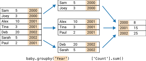
(A depiction of grouping and then aggregating for example data)
We call this operation grouping followed by aggregating. In pandas, we write:
baby.groupby('Year')['Count'].sum()
Year
1880     194419
1881     185772
1882     213385
1883     208932
1884     234244
         ...
2016    3642755
2017    3548457
2018    3487193
2019    3437438
2020    3287724
Name: Count, Length: 141, dtype: int64
Notice that the code is nearly the same as the nongrouped version, except that it starts with a call to .groupby('Year').
The result is a pd.Series with the total number of babies born for each year in the
data. Notice that the index of this series contains the unique Year values. Now we can plot the counts over time:
counts_by_year = baby.groupby('Year')['Count'].sum().reset_index()
fig, ax = subplots(figsize=(7, 4))
ax.plot(counts_by_year['Year'], counts_by_year['Count'])
ax.set_xlabel('Year')
ax.set_ylabel('Count')
Text(0, 0.5, 'Count')

What do we see in this plot? First, we notice that there seem to be suspiciously few babies born before 1920. One likely explanation is that the SSA was created in 1935, so its data for prior births could be less complete.
We also notice the dip when World War II began in 1939, and the post-war baby boomer era from 1946 to 1964.
Here's the basic recipe for grouping in pandas:
(baby                # the dataframe
 .groupby('Year')    # column(s) to group
 ['Count']           # column(s) to aggregate
 .sum()              # how to aggregate
)
Example: Using .value_counts()
One of the more common dataframe tasks is to count the number of times every unique item in a column appears. For example, we might be interested in the number of times each name appears in the following classroom dataframe:
classroom = pd.DataFrame({
    'name': ['Eden', 'Sachit', 'Eden', 'Sachit', 'Sachit', 'Luke'],
})
classroom
| name | |
|---|---|
| 0 | Eden |
| 1 | Sachit |
| 2 | Eden |
| 3 | Sachit |
| 4 | Sachit |
| 5 | Luke |
One way to do this is to use our grouping recipe with the .size() aggregation function:
(
    classroom.groupby('name')['name'].size()
)
name
Eden      2
Luke      1
Sachit    3
Name: name, dtype: int64
This operation is so common that pandas provides a shorthand—the .value_counts() method for pd.Series objects:
classroom['name'].value_counts()
name
Sachit    3
Eden      2
Luke      1
Name: count, dtype: int64
By default, the .value_counts() method will sort the resulting series from highest to lowest number, making it convenient to see the most and least common values. We point out this method because we use it often in other chapters of the book.
Grouping on Multiple Columns
We pass multiple columns into .groupby as a list to group by multiple
columns at once. This is useful when we need to further subdivide our groups.
For example, we can group by both year and sex to see how many male and female
babies were born over time:
counts_by_year_and_sex = (baby
 .groupby(['Year', 'Sex']) # Arg to groupby is a list of column names
 ['Count']
 .sum()
)
counts_by_year_and_sex
Year  Sex
1880  F        83929
      M       110490
1881  F        85034
      M       100738
1882  F        99699
              ...
2018  M      1810309
2019  F      1651911
      M      1785527
2020  F      1581301
      M      1706423
Name: Count, Length: 282, dtype: int64
Notice how the code closely follows the grouping recipe.
The counts_by_year_and_sex series has what we call a multilevel index with
two levels, one for each column that was grouped. It's a bit easier to see if
we convert the series to a dataframe:
# The result only has one column.
counts_by_year_and_sex.to_frame()
| Count | ||
|---|---|---|
| Year | Sex | |
| 1880 | F | 83929 |
| M | 110490 | |
| 1881 | F | 85034 |
| M | 100738 | |
| 1882 | F | 99699 |
| ... | ... | ... |
| 2018 | M | 1810309 |
| 2019 | F | 1651911 |
| M | 1785527 | |
| 2020 | F | 1581301 |
| M | 1706423 |
282 rows × 1 columns
There are two levels to the index because we grouped by two columns. It can be a bit tricky to work with multilevel indices, so we can reset the index to go back to a dataframe with a single index:
counts_by_year_and_sex.reset_index()
| Year | Sex | Count | |
|---|---|---|---|
| 0 | 1880 | F | 83929 |
| 1 | 1880 | M | 110490 |
| 2 | 1881 | F | 85034 |
| 3 | 1881 | M | 100738 |
| 4 | 1882 | F | 99699 |
| ... | ... | ... | ... |
| 277 | 2018 | M | 1810309 |
| 278 | 2019 | F | 1651911 |
| 279 | 2019 | M | 1785527 |
| 280 | 2020 | F | 1581301 |
| 281 | 2020 | M | 1706423 |
282 rows × 3 columns
Custom Aggregation Functions
After grouping, pandas gives us flexible ways to aggregate the data. So far,
we've seen how to use .sum() after grouping:
(baby
 .groupby('Year')
 ['Count']
 .sum() # aggregate by summing
)
Year
1880     194419
1881     185772
1882     213385
1883     208932
1884     234244
         ...
2016    3642755
2017    3548457
2018    3487193
2019    3437438
2020    3287724
Name: Count, Length: 141, dtype: int64
pandas also supplies other aggregation functions, like .mean(), .size(),
and .first(). Here's the same grouping using .max():
(baby
 .groupby('Year')
 ['Count']
 .max() # aggregate by taking the max within each group
)
Year
1880     9655
1881     8769
1882     9557
1883     8894
1884     9388
        ...
2016    19380
2017    18824
2018    19924
2019    20555
2020    19659
Name: Count, Length: 141, dtype: int64
But sometimes pandas doesn't have the exact aggregation function we want to use. In these cases, we can define and use a custom aggregation function. pandas lets us do this through .agg(fn), where fn is a function that we define.
For instance, if we want to find the difference between the largest and smallest values within each group (the range of the data), we could first define a function called data_range, then pass that function into .agg():
# The input to this function is a pd.Series object containing a single column
# of data. It gets called once for each group.
def data_range(counts):
    return counts.max() - counts.min()

(baby
 .groupby('Year')
 ['Count']
 .agg(data_range) # aggregate using custom function
)
Year
1880     9650
1881     8764
1882     9552
1883     8889
1884     9383
        ...
2016    19375
2017    18819
2018    19919
2019    20550
2020    19654
Name: Count, Length: 141, dtype: int64
We start by defining a count_unique function that counts the number of
unique values in a series. Then we pass that function into .agg():
# Since this function is short, we could use a lambda instead
def count_unique(s):
    return len(s.unique())

unique_names_by_year = (baby
 .groupby('Year')
 ['Name']
 .agg(count_unique) # aggregate using the custom count_unique function
)
unique_names_by_year
Year
1880     1889
1881     1829
1882     2012
1883     1962
1884     2158
        ...
2016    30431
2017    30042
2018    29619
2019    29417
2020    28613
Name: Name, Length: 141, dtype: int64
unique_names_by_year = unique_names_by_year.reset_index()
fig, ax = subplots(figsize=(7, 5))
ax.plot(unique_names_by_year['Year'], unique_names_by_year['Name'])
ax.set_xlabel('Year')
ax.set_ylabel('# Unique Names')
Text(0, 0.5, '# Unique Names')

We see that the number of unique names has generally increased over time, even though the number of babies born annually has plateaued since the 1960s.
Pivoting
Pivoting is essentially a convenient way to arrange the results of a group and aggregation when grouping with two columns. Earlier in this section we grouped the baby names data by year and sex:
counts_by_year_and_sex = (baby
 .groupby(['Year', 'Sex'])
 ['Count']
 .sum()
)
counts_by_year_and_sex.to_frame()
| Count | ||
|---|---|---|
| Year | Sex | |
| 1880 | F | 83929 |
| M | 110490 | |
| 1881 | F | 85034 |
| M | 100738 | |
| 1882 | F | 99699 |
| ... | ... | ... |
| 2018 | M | 1810309 |
| 2019 | F | 1651911 |
| M | 1785527 | |
| 2020 | F | 1581301 |
| M | 1706423 |
282 rows × 1 columns
This produces a pd.Series with the counts. We can also imagine the same data with the Sex index level "pivoted" to the columns of a dataframe. It's easier to see with an example:
mf_pivot = pd.pivot_table(
    baby,
    index='Year',   # Column to turn into new index
    columns='Sex',  # Column to turn into new columns
    values='Count', # Column to aggregate for values
    aggfunc=sum)    # Aggregation function
mf_pivot
/var/folders/_d/hkwrjflx01l0hnh4x90j7ct40000gn/T/ipykernel_37809/3000549939.py:1: FutureWarning: The provided callable <built-in function sum> is currently using DataFrameGroupBy.sum. In a future version of pandas, the provided callable will be used directly. To keep current behavior pass the string "sum" instead.
  mf_pivot = pd.pivot_table(
| Sex | F | M |
|---|---|---|
| Year | ||
| 1880 | 83929 | 110490 |
| 1881 | 85034 | 100738 |
| 1882 | 99699 | 113686 |
| 1883 | 104307 | 104625 |
| 1884 | 119802 | 114442 |
| ... | ... | ... |
| 2016 | 1748838 | 1893917 |
| 2017 | 1702303 | 1846154 |
| 2018 | 1676884 | 1810309 |
| 2019 | 1651911 | 1785527 |
| 2020 | 1581301 | 1706423 |
141 rows × 2 columns
Notice that the data values are identical in the pivot table and the table produced with .groupby(); the values are just arranged differently. Pivot tables are useful for quickly summarizing data using two attributes and are often seen in articles and papers.
We can plot year-wise data on the number of 'M' and 'F' on the same plot.
mf_pivot = mf_pivot.reset_index()
fig, ax = subplots(figsize=(7, 5))
ax.plot(mf_pivot['Year'], mf_pivot['M'], label='M')
ax.plot(mf_pivot['Year'], mf_pivot['F'], label='F')
ax.set_xlabel('Year')
ax.set_ylabel('#')
ax.legend()
<matplotlib.legend.Legend at 0x10e29ebb0>

This section covered common ways to aggregate data in pandas using the .groupby() function with one or more columns, or using the pd.pivot_table() function. In the next section, we'll explain how to join dataframes together.
2.3. Joining
Data scientists very frequently want to join two or more dataframes together in order to connect data values across dataframes. For instance, an online bookstore might have one dataframe with the books each user has ordered and a second dataframe with the genres of each book. By joining the two dataframes together, the data scientist can see what genres each user prefers.
We'll continue looking at the baby names data. We'll use joins to check some trends mentioned in the [New York Times article about baby names (https://www.nytimes.com/2021/06/12/style/lilibet-popular-baby-names.html). The article talks about how certain categories of names have become more or less popular over time. For instance, it mentions that mythological names like Julius and Cassius have become popular, while baby boomer names like Susan and Debbie have become less popular. How has the popularity of these categories changed over time?
We've taken the names and categories in the NYT article and put them in a small dataframe:
nyt = pd.read_csv('nyt_names.csv')
nyt
| nyt_name | category | |
|---|---|---|
| 0 | Lucifer | forbidden |
| 1 | Lilith | forbidden |
| 2 | Danger | forbidden |
| 3 | Amen | evangelical |
| 4 | Savior | evangelical |
| 5 | Canaan | evangelical |
| 6 | Creed | evangelical |
| 7 | Saint | evangelical |
| 8 | Susan | boomer |
| 9 | Debbie | boomer |
| 10 | Bobby | boomer |
| 11 | Karen | boomer |
| 12 | Julius | mythology |
| 13 | Cassius | mythology |
| 14 | Freya | mythology |
| 15 | Hera | mythology |
| 16 | Nyx | mythology |
| 17 | Osiris | mythology |
| 18 | Onyx | mineral |
| 19 | Amethyst | mineral |
| 20 | Venus | celestial |
| 21 | Celestia | celestial |
| 22 | Skye | celestial |
To see how popular the categories of names are, we join the nyt dataframe with the baby dataframe to get the name counts from baby:
baby
| Name | Sex | Count | Year | |
|---|---|---|---|---|
| 0 | Liam | M | 19659 | 2020 |
| 1 | Noah | M | 18252 | 2020 |
| 2 | Oliver | M | 14147 | 2020 |
| 3 | Elijah | M | 13034 | 2020 |
| 4 | William | M | 12541 | 2020 |
| ... | ... | ... | ... | ... |
| 2020717 | Ula | F | 5 | 1880 |
| 2020718 | Vannie | F | 5 | 1880 |
| 2020719 | Verona | F | 5 | 1880 |
| 2020720 | Vertie | F | 5 | 1880 |
| 2020721 | Wilma | F | 5 | 1880 |
2020722 rows × 4 columns
For intuition, we can imagine going down each row in baby and asking: is this name in the nyt table? If so, then add the value in the category column to the row. This is the basic idea behind a join. Let's look at a few examples on smaller dataframes first.
Inner Joins
We start by making smaller versions of the baby and nyt tables so that it's easier to see what happens when we join tables together:
nyt_small = nyt.iloc[[11, 12, 14]].reset_index(drop=True)

names_to_keep = ['Julius', 'Karen', 'Noah']
baby_small = (baby
 .query("Year == 2020 and Name in @names_to_keep")
 .reset_index(drop=True)
)
nyt_small
| nyt_name | category | |
|---|---|---|
| 0 | Karen | boomer |
| 1 | Julius | mythology |
| 2 | Freya | mythology |
baby_small
| Name | Sex | Count | Year | |
|---|---|---|---|---|
| 0 | Noah | M | 18252 | 2020 |
| 1 | Julius | M | 960 | 2020 |
| 2 | Karen | M | 6 | 2020 |
| 3 | Karen | F | 325 | 2020 |
| 4 | Noah | F | 305 | 2020 |
To join tables in pandas, we'll use the .merge() method:
baby_small.merge(nyt_small,
                 left_on='Name',        # column in left table to match
                 right_on='nyt_name')   # column in right table to match
| Name | Sex | Count | Year | nyt_name | category | |
|---|---|---|---|---|---|---|
| 0 | Julius | M | 960 | 2020 | Julius | mythology |
| 1 | Karen | M | 6 | 2020 | Karen | boomer |
| 2 | Karen | F | 325 | 2020 | Karen | boomer |
When we join two tables together, we tell pandas the column(s) from each table that we want to use to make the join (the left_on and right_on arguments). pandas matches rows together when the values in the joining columns match, as shown in the figure below.
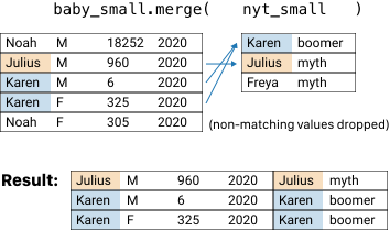
(To join, pandas matches rows using the values in the Name and nyt_name columns, dropping rows that don't have matching values)
By default, pandas does an inner join. If either table has rows that don't have matches in the other table, pandas drops those rows from the result. In this case, the Noah rows in baby_small don't have matches in nyt_small, so they are dropped. Also, the Freya row in nyt_small doesn't have matches in baby_small, so it's dropped as well. Only the rows with a match in both tables stay in the final result.
Left, Right, and Outer Joins
We sometimes want to keep rows without a match instead of dropping them entirely. There are other types of joins---left, right, and outer---that keep rows even when they don't have a match.
In a left join, rows in the left table without a match are kept in the final result, as shown in the figure below.
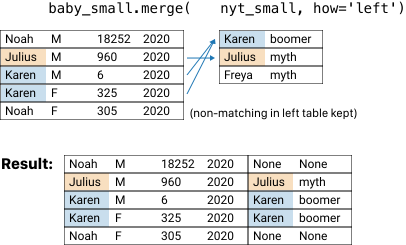
(In a left join, rows in the left table that don't have matching values are kept)
To do a left join in pandas, use how='left' in the call to .merge():
baby_small.merge(nyt_small,
                 left_on='Name',
                 right_on='nyt_name',
                 how='left')           # left join instead of inner
| Name | Sex | Count | Year | nyt_name | category | |
|---|---|---|---|---|---|---|
| 0 | Noah | M | 18252 | 2020 | NaN | NaN |
| 1 | Julius | M | 960 | 2020 | Julius | mythology |
| 2 | Karen | M | 6 | 2020 | Karen | boomer |
| 3 | Karen | F | 325 | 2020 | Karen | boomer |
| 4 | Noah | F | 305 | 2020 | NaN | NaN |
Notice that the Noah rows are kept in the final table. Since those rows didn't have a match in the nyt_small dataframe, the join leaves NaN values in the nyt_name and category columns. Also, notice that the Freya row in nyt_small is still dropped.
A right join works similarly to the left join, except that nonmatching rows in the right table are kept instead of the left table:
baby_small.merge(nyt_small,
                 left_on='Name',
                 right_on='nyt_name',
                 how='right')
| Name | Sex | Count | Year | nyt_name | category | |
|---|---|---|---|---|---|---|
| 0 | Karen | M | 6.0 | 2020.0 | Karen | boomer |
| 1 | Karen | F | 325.0 | 2020.0 | Karen | boomer |
| 2 | Julius | M | 960.0 | 2020.0 | Julius | mythology |
| 3 | NaN | NaN | NaN | NaN | Freya | mythology |
Finally, an outer join keeps rows from both tables even when they don't have a match:
baby_small.merge(nyt_small,
                 left_on='Name',
                 right_on='nyt_name',
                 how='outer')
| Name | Sex | Count | Year | nyt_name | category | |
|---|---|---|---|---|---|---|
| 0 | NaN | NaN | NaN | NaN | Freya | mythology |
| 1 | Julius | M | 960.0 | 2020.0 | Julius | mythology |
| 2 | Karen | M | 6.0 | 2020.0 | Karen | boomer |
| 3 | Karen | F | 325.0 | 2020.0 | Karen | boomer |
| 4 | Noah | M | 18252.0 | 2020.0 | NaN | NaN |
| 5 | Noah | F | 305.0 | 2020.0 | NaN | NaN |
Example: Popularity of NYT Name Categories
Now let's return to the full dataframes baby and nyt:
# .head() slices out the first few rows - convenient for saving space
baby.head(2)
| Name | Sex | Count | Year | |
|---|---|---|---|---|
| 0 | Liam | M | 19659 | 2020 |
| 1 | Noah | M | 18252 | 2020 |
nyt.head(2)
| nyt_name | category | |
|---|---|---|
| 0 | Lucifer | forbidden |
| 1 | Lilith | forbidden |
We want to know how the popularity of name categories in nyt has changed
over time. To answer this question:
- Inner join
babywithnyt. - Group the table by
categoryandYear. - Aggregate the counts using a sum:
cate_counts = (
    baby.merge(nyt, left_on='Name', right_on='nyt_name') # [1]
    .groupby(['category', 'Year'])                       # [2]
    ['Count']                                            # [3]
    .sum()                                               # [3]
    .reset_index()
)
cate_counts
| category | Year | Count | |
|---|---|---|---|
| 0 | boomer | 1880 | 292 |
| 1 | boomer | 1881 | 298 |
| 2 | boomer | 1882 | 326 |
| 3 | boomer | 1883 | 322 |
| 4 | boomer | 1884 | 335 |
| ... | ... | ... | ... |
| 645 | mythology | 2016 | 2671 |
| 646 | mythology | 2017 | 2797 |
| 647 | mythology | 2018 | 2944 |
| 648 | mythology | 2019 | 3320 |
| 649 | mythology | 2020 | 3489 |
650 rows × 3 columns
Now we can plot the popularity of boomer names and mythology names:
boomers = cate_counts.query('category == "boomer"')
myths = cate_counts.query('category == "mythology"')

# Create a figure and a set of subplots (1 row, 2 columns)
fig, (ax1, ax2) = subplots(1, 2, figsize = (8, 4)) #

# Plot data on the first axis (left plot)
ax1.plot(boomers['Year'], boomers['Count'])
ax1.set_title('Boomer names')
ax1.set_xlabel('Year')


# Plot data on the second axis (right plot)
ax2.plot(myths['Year'], myths['Count'])
ax2.set_title('Mythology names')
ax2.set_xlabel('Year')
Text(0.5, 0, 'Year')

As the NYT article claims, baby boomer names have become less popular since 2000, while mythology names have become more popular.
We can also plot the popularity of all the categories at once. Take a look at the following plots and see whether they support the claims made in the New York Times article. First, let us find out the categories.
cate_counts['category'].unique()
array(['boomer', 'celestial', 'evangelical', 'forbidden', 'mineral',
       'mythology'], dtype=object)
boomer = cate_counts.query('category == "boomer"')
celestial = cate_counts.query('category == "celestial"')
evangelical = cate_counts.query('category == "evangelical"')
forbidden = cate_counts.query('category == "forbidden"')
mineral = cate_counts.query('category == "mineral"')
mythology = cate_counts.query('category == "mythology"')

# Create a figure and a set of subplots (2 row, 3 columns)
fig, ax = subplots(2, 3, figsize = (12, 8)) #

ax[0, 0].plot(boomer['Year'], boomer['Count'])
ax[0, 0].set_title('Boomer names')
ax[0, 0].set_xlabel('Year')

ax[0, 1].plot(celestial['Year'], celestial['Count'])
ax[0, 1].set_title('Celestial names')
ax[0, 1].set_xlabel('Year')

ax[0, 2].plot(evangelical['Year'], evangelical['Count'])
ax[0, 2].set_title('Evangelical names')
ax[0, 2].set_xlabel('Year')

ax[1, 0].plot(forbidden['Year'], forbidden['Count'])
ax[1, 0].set_title('Forbidden names')
ax[1, 0].set_xlabel('Year')

ax[1, 1].plot(mineral['Year'], mineral['Count'])
ax[1, 1].set_title('Mineral names')
ax[1, 1].set_xlabel('Year')

ax[1, 2].plot(mythology['Year'], mythology['Count'])
ax[1, 2].set_title('Mythology names')
ax[1, 2].set_xlabel('Year')

fig.tight_layout()

In this section, we introduced joins for dataframes. When joining dataframes together, we match rows using the .merge() function. It's important to consider the type of join (inner, left, right, or outer) when joining dataframes. In the next section, we'll explain how to transform values in a dataframe.
2.4. Transforming
Data scientists transform dataframe columns when they need to change each value in a feature in the same way. For example, if a feature contains heights of people in feet, a data scientist might want to transform the heights to centimeters. In this section, we'll introduce apply, an operation that transforms columns of data using a user-defined function:
baby
| Name | Sex | Count | Year | |
|---|---|---|---|---|
| 0 | Liam | M | 19659 | 2020 |
| 1 | Noah | M | 18252 | 2020 |
| 2 | Oliver | M | 14147 | 2020 |
| 3 | Elijah | M | 13034 | 2020 |
| 4 | William | M | 12541 | 2020 |
| ... | ... | ... | ... | ... |
| 2020717 | Ula | F | 5 | 1880 |
| 2020718 | Vannie | F | 5 | 1880 |
| 2020719 | Verona | F | 5 | 1880 |
| 2020720 | Vertie | F | 5 | 1880 |
| 2020721 | Wilma | F | 5 | 1880 |
2020722 rows × 4 columns
In the baby names New York Times article, Pamela
mentions that names starting with the letter L or K became popular
after 2000. On the other hand, names starting with the letter J peaked in
popularity in the 1970s and 1980s and dropped off in popularity since. We
can verify these claims using the baby dataset.
We approach this problem using the following steps:
- Transform the
Namecolumn into a new column that contains the first letters of each value inName. - Group the dataframe by the first letter and year.
- Aggregate the name counts by summing.
To complete the first step, we'll apply a function to the Name column.
Apply
pd.Series objects contain an .apply() method that takes in a function and applies it to each value in the series. For instance, to find the lengths of each name, we apply the len function:
names = baby['Name']
names.apply(len)
0          4
1          4
2          6
3          6
4          7
          ..
2020717    3
2020718    6
2020719    6
2020720    6
2020721    5
Name: Name, Length: 2020722, dtype: int64
To extract the first letter of each name, we define a custom function and pass it into .apply():
# The argument to the function is an individual value in the series.
def first_letter(string):
    return string[0]

names.apply(first_letter)
0          L
1          N
2          O
3          E
4          W
          ..
2020717    U
2020718    V
2020719    V
2020720    V
2020721    W
Name: Name, Length: 2020722, dtype: object
Using .apply() is similar to using a for loop. The preceding code is roughly
equivalent to writing:
result = []
for name in names:
    result.append(first_letter(name))
Now we can assign the first letters to a new column in the dataframe:
letters = baby.assign(Firsts=names.apply(first_letter))
letters
| Name | Sex | Count | Year | Firsts | |
|---|---|---|---|---|---|
| 0 | Liam | M | 19659 | 2020 | L |
| 1 | Noah | M | 18252 | 2020 | N |
| 2 | Oliver | M | 14147 | 2020 | O |
| 3 | Elijah | M | 13034 | 2020 | E |
| 4 | William | M | 12541 | 2020 | W |
| ... | ... | ... | ... | ... | ... |
| 2020717 | Ula | F | 5 | 1880 | U |
| 2020718 | Vannie | F | 5 | 1880 | V |
| 2020719 | Verona | F | 5 | 1880 | V |
| 2020720 | Vertie | F | 5 | 1880 | V |
| 2020721 | Wilma | F | 5 | 1880 | W |
2020722 rows × 5 columns
baby['Firsts'] = names.apply(first_letter)
This mutates the baby table by adding a new column called Firsts. In the preceding
code, we use .assign(), which doesn't mutate the baby table itself; it
creates a new dataframe instead. Mutating dataframes isn't wrong but can be a
common source of bugs. Because of this, we'll mostly use .assign() in this
book.
Example: Popularity of "L" Names
Now we can use the letters dataframe to see the popularity of first letters over time:
letter_counts = (letters
 .groupby(['Firsts', 'Year'])
 ['Count']
 .sum()
 .reset_index()
)
letter_counts
| Firsts | Year | Count | |
|---|---|---|---|
| 0 | A | 1880 | 16740 |
| 1 | A | 1881 | 16257 |
| 2 | A | 1882 | 18790 |
| 3 | A | 1883 | 18831 |
| 4 | A | 1884 | 20898 |
| ... | ... | ... | ... |
| 3636 | Z | 2016 | 54679 |
| 3637 | Z | 2017 | 54495 |
| 3638 | Z | 2018 | 55996 |
| 3639 | Z | 2019 | 55293 |
| 3640 | Z | 2020 | 54011 |
3641 rows × 3 columns
lnames = letter_counts.query('Firsts == "L"')

fig, ax = subplots(figsize = (4, 4))
ax.plot(lnames['Year'], lnames['Count'])
ax.set_xlabel('Year')
ax.set_ylabel('Count')
Text(0, 0.5, 'Count')

The plot shows that "L" names were popular in the 1960s, dipped in the decades after, but have indeed resurged in popularity since 2000.
What about "J" names?
jnames = letter_counts.query('Firsts == "J"')

fig, ax = subplots(figsize = (4, 4))
ax.plot(jnames['Year'], jnames['Count'])
ax.set_xlabel('Year')
ax.set_ylabel('Count')
Text(0, 0.5, 'Count')

The NYT article says that "J" names were popular in the 1970s and '80s. The plot agrees and shows that they have become less popular since 2000.
The Price of Apply
The power of .apply() is its flexibility---you can call it with any function that takes in a single data value and outputs a single data value.
Its flexibility has a price, though. Using .apply() can be slow, since pandas can't optimize arbitrary functions. For example, using .apply() for numeric calculations is much slower than using vectorized operations directly on pd.Series objects:
%%timeit

# Calculate the decade using vectorized operators
baby['Year'] // 10 * 10
2.08 ms ± 5.36 µs per loop (mean ± std. dev. of 7 runs, 100 loops each)
%%timeit

def decade(yr):
    return yr // 10 * 10

# Calculate the decade using apply
baby['Year'].apply(decade)
322 ms ± 1.7 ms per loop (mean ± std. dev. of 7 runs, 1 loop each)
The version using .apply() is much slower! For numeric operations in particular, we recommend operating on pd.Series objects directly.
In this section, we introduced data transformations. To transform values in a dataframe, we commonly use the .apply() and .assign() functions. In the next section, we'll compare dataframes with other ways to represent and manipulate data tables.
2.5. How Are Dataframes Different from Other Data Representations?
Dataframes are just one way to represent data stored in a table. In practice, data scientists encounter many other types of data tables, like spreadsheets, matrices, and relations. In this section, we'll compare and contrast the dataframe with other representations to explain why dataframes have become so widely used for data analysis. We'll also point out scenarios where other representations might be more appropriate.
Dataframes and Spreadsheets
Spreadsheets are computer applications in which users can enter data in a grid and use formulas to perform calculations. One well-known example today is Microsoft Excel, although spreadsheets date back to at least 1979 with [VisiCalc (https://doi.org/10.1109/MAHC.2007.4338439). Spreadsheets make it easy to see and directly manipulate data since spreadsheet formulas can automatically recalculate results whenever the data change. In contrast, dataframe code typically needs to be manually rerun when datasets are updated. These properties make spreadsheets highly popular---by a 2005 estimate, there are over 55 million spreadsheet users compared to 3 million professional programmers in industry.
Dataframes have several key advantages over spreadsheets. Writing dataframe code in a computational notebook like Jupyter naturally produces a data lineage. Someone who opens the notebook can see the input files for the notebook and how the data were changed. Spreadsheets do not make a data lineage visible; if a person manually edits data values in a cell, it can be difficult for future users to see which values were manually edited and how they were edited. Dataframes can handle larger datasets than spreadsheets, and users can also use distributed programming tools to work with huge datasets that would be very hard to load into a spreadsheet.
Dataframes and Matrices
A matrix is a two-dimensional array of data used primarily for linear algebra operations. In this next example, $ \mathbf{X} $ is a matrix with three rows and two columns:
$$ \begin{aligned} \mathbf{X} = \begin{bmatrix} 1 & 0 \\ 0 & 4 \\ 0 & 0 \\ \end{bmatrix} \end{aligned} $$
Matrices are mathematical objects defined by the operators that they allow. For instance, matrices can be added or multiplied together. Matrices also have a transpose. These operators have very useful properties that data scientists rely on for statistical modeling.
One important difference between a matrix and a dataframe is that when matrices are treated as mathematical objects, they can only contain numbers. Dataframes, on the other hand, can also have other types of data, like text. This makes dataframes more useful for loading and processing raw data that may contain all kinds of data types. In practice, data scientists often load data into dataframes, then manipulate the data into matrix form. In this book, we'll generally use dataframes for exploratory data analysis and data cleaning, then process the data into matrices for machine learning models.
Dataframes and Relations
A relation is a data table representation used in database systems, especially SQL systems like SQLite and PostgreSQL. Relations share many similarities with dataframes; both use rows to represent records and columns to represent features. Both have column names, and data within a column have the same type.
One key advantage of dataframes is that they don't require rows to represent records and columns to represent features. Many times, raw data don't come in a convenient format that can directly be put into a relation. In these scenarios, data scientists use the dataframe to load and process data since dataframes are more flexible in this regard. Often, data scientists will load raw data into a dataframe, then process the data into a format that can easily be stored into a relation.
One key advantage that relations have over dataframes is that relations are
used by relational database systems like PostgreSQL that have highly
useful features for data storage and management. Consider a data scientist at a
company that runs a large social media website. The database might hold data
that is far too large to read into a pandas dataframe all at once; instead,
data scientists use SQL queries to subset and aggregate data since database
systems are more capable of handling large datasets. Also, website users
constantly make updates to their data by making posts, uploading pictures, and
editing their profile. Here, database systems let data scientists reuse their
existing SQL queries to update their analyses with the latest data rather than
having to repeatedly download large CSV files.
2.6. Summary
In this chapter, we explained what dataframes are, why they're useful, and how to work with them using pandas code. Subsetting, aggregating, joining, and transforming are
useful in nearly every data analysis. We'll rely on these operations often in the rest of the course.