Lab-11 (SVD)

(Intro. to Data Science: IIT Delhi - Abu Dhabi)

In this lab, we study how SVD (in particular, Truncated SVD) can help $k$-nearest neighbors classification on high-dimensional text data. We then explore other applications of SVD: topic discovery, image compression, noise reduction, and latent-factor models for recommendation.

Learning goals: By the end of this lab, you should be able to:

1. Explain why high-dimensional sparse text data can be difficult for k-NN.
2. Build a TF-IDF + k-NN text classifier.
3. Use Truncated SVD to reduce the dimension of sparse text data.
4. Compare k-NN before and after dimensionality reduction.
5. Tune the number of SVD components.
6. Interpret SVD components as latent semantic directions.
7. Use SVD for image compression, noise reduction, and simple recommendation-style latent factors.

11.1 Background theory:

SVD

For a data matrix $X \in \mathbb{R}^{n \times p},$ the singular value decomposition is $X = U \Sigma V^T.$ The rank-$k$ truncated SVD approximation keeps only the top $k$ singular values: $X \approx X_k = U_k \Sigma_k V_k^T.$

Processing Text data using TF-IDF

Machine learning algorithms usually require numerical input, but text data comes in the form of words and documents. Therefore, before applying algorithms such as logistic regression, k-nearest neighbors, support vector machines, or clustering methods, we need to convert text into numerical feature vectors. One common and effective method for doing this is TF-IDF, which stands for Term Frequency–Inverse Document Frequency.

TF-IDF assigns a numerical weight to each word in each document. The weight is high when a word appears frequently in a particular document, but does not appear too often across the entire collection of documents. In other words, TF-IDF tries to identify words that are important for distinguishing one document from others.

Suppose we have a collection of documents. The term frequency part measures how often a term appears in a document. If a word appears many times in a document, it may be important for that document. For example, in a document about space science, words such as “orbit,” “rocket,” and “planet” may appear frequently.

However, some words appear frequently in almost all documents. Words such as “the,” “is,” “and,” and “of” are common, but they usually do not help us understand the specific topic of a document. This is where the inverse document frequency part is useful. It gives lower weight to words that appear in many documents and higher weight to words that appear in relatively few documents.

A common formula for TF-IDF is: $$\text{TF-IDF}(t, d) = TF(t, d) \times IDF(t),$$ where $t$ is a term and $d$ is a document. The inverse document frequency is often written as: $$\text{IDF}(t) = \log{\left( \frac{N}{df(t)}\right)}, $$ where $N$ is the total number of documents and $df(t)$ is the number of documents containing term $t$. So TF-IDF captures two ideas at the same time: $$\text{important word} = \text{frequent in this document} \times \text{rare across documents}$$

After applying TF-IDF, a text dataset becomes a matrix. Each row represents a document, each column represents a word or term, and each entry contains the TF-IDF score of that word in that document. For example: $$X_{ij} = \text{TF-IDF score of word $j$ in document $i$}$$ This matrix can then be used as input to machine learning algorithms. For text data, the matrix $X$ is often a sparse TF-IDF document-term matrix.

A typical text-processing workflow is:

1. Collect a set of documents.
2. Clean the text by removing unnecessary characters, punctuation, or HTML tags.
3. Convert all text to lowercase.
4. Remove very common words, often called stop words.
5. Convert the documents into a TF-IDF matrix.
6. Use the TF-IDF matrix in a machine learning model.

In Python, text processing can be done using scikit-learn:

from sklearn.feature_extraction.text import TfidfVectorizer

documents = [
    "space rocket mission",
    "space telescope orbit",
    "baseball team game"
]

vectorizer = TfidfVectorizer(stop_words="english")
X = vectorizer.fit_transform(documents)

print(vectorizer.get_feature_names_out())
print(X.toarray())

The output matrix contains numerical representations of the documents. Words that are more distinctive for a document receive larger values.

TF-IDF is especially useful in tasks such as document classification, spam detection, sentiment analysis, search engines, and clustering. For example, in document classification, a model can use TF-IDF features to learn that words such as “orbit” and “rocket” are associated with space-related documents, while words such as “team” and “game” may be associated with sports-related documents.

One important point is that TF-IDF matrices are often very high-dimensional and sparse. This means there may be thousands or tens of thousands of possible words, but each document contains only a small fraction of them. Because of this, TF-IDF is often combined with dimensionality reduction methods such as Truncated SVD before applying algorithms like k-nearest neighbors or clustering. Truncated SVD gives each document a lower-dimensional representation: $Z = U_k \Sigma_k.$ Then we can run predictors such as k-NN on $Z$ instead of the original high-dimensional TF-IDF matrix.

In summary, TF-IDF is a method for converting text into numerical data by giving high weight to words that are frequent in a document but rare across the collection. It is a simple, powerful, and widely used representation for text-based machine learning.

With that background, let's now continue with our lab. We start with importing all the relevant modules.

import time
import numpy as np
import pandas as pd
import matplotlib.pyplot as plt

from sklearn.datasets import fetch_20newsgroups, load_sample_image
from sklearn.feature_extraction.text import TfidfVectorizer
from sklearn.decomposition import TruncatedSVD
from sklearn.preprocessing import Normalizer
from sklearn.pipeline import Pipeline
from sklearn.neighbors import KNeighborsClassifier
from sklearn.linear_model import LogisticRegression
from sklearn.metrics import accuracy_score, classification_report, confusion_matrix, ConfusionMatrixDisplay

RANDOM_STATE = 42

Most of the above modules and functions must be familiar to you by now. There are a few that we may not have seen before (e.g., sklearn.Normalizer). These will come up naturally in our discussion. First, we load the data that we shall be working with.

We use the 20 Newsgroups dataset (link), a classic text-classification dataset. To keep the lab fast, we begin with four categories. You can later try all 20 categories as an extension.

categories = [
    "comp.graphics",
    "sci.space",
    "rec.sport.baseball",
    "talk.politics.misc"
]

train = fetch_20newsgroups(
    subset="train",
    categories=categories,
    remove=("headers", "footers", "quotes"),
    random_state=RANDOM_STATE
)

test = fetch_20newsgroups(
    subset="test",
    categories=categories,
    remove=("headers", "footers", "quotes"),
    random_state=RANDOM_STATE
)

y_train = train.target
y_test = test.target

print("Training documents:", len(train.data))
print("Test documents:", len(test.data))
print("Classes:", train.target_names)

# Let us examine a few of the data elements
for i in range(3):
    print("=" * 80)
    print("Class:", train.target_names[y_train[i]])
    print(train.data[i][:150])

We transform documents into TF-IDF vectors. A TF-IDF matrix has one row per document and one column per term. These matrices are usually high-dimensional, sparse, and nonnegative.

# Please read the documentation of the TfidfVectorizer to understand some of the input parameters
tfidf = TfidfVectorizer(
    stop_words="english", # This is to exclude common words such as "the, a, an"
    min_df=3, # This is to exclude rare words
    max_df=0.8 # This is to exclude extremely common words
)

X_train = tfidf.fit_transform(train.data)
X_test = tfidf.transform(test.data)

print("X_train shape:", X_train.shape)
print("X_test shape:", X_test.shape)
print("Number of stored nonzero entries:", X_train.nnz)
print("Sparsity percentage:", 100 * (1 - X_train.nnz / (X_train.shape[0] * X_train.shape[1])))

We now train a k-NN classifier directly on the TF-IDF vectors. For TF-IDF vectors, cosine distance is often more meaningful than Euclidean distance because document length and direction matter.

knn_baseline = KNeighborsClassifier(
    n_neighbors=5,
    metric="cosine"
)

start = time.time()
knn_baseline.fit(X_train, y_train)
fit_time_baseline = time.time() - start

start = time.time()
y_pred_baseline = knn_baseline.predict(X_test)
pred_time_baseline = time.time() - start

acc_baseline = accuracy_score(y_test, y_pred_baseline)

print("Baseline TF-IDF + k-NN accuracy:", acc_baseline)
print("Fit time:", fit_time_baseline)
print("Prediction time:", pred_time_baseline)
print()
print(classification_report(y_test, y_pred_baseline, target_names=test.target_names))

cm = confusion_matrix(y_test, y_pred_baseline)
disp = ConfusionMatrixDisplay(cm, display_labels=test.target_names)
disp.plot(xticks_rotation=45)
plt.title("Baseline TF-IDF + k-NN")
plt.show()

Truncated SVD:

Now we insert Truncated SVD into the pipeline. Let us go over a short tutorial on Truncated SVD before moving on.

Suppose your data matrix is $X \in \mathbb{R}^{n\times p}$, where $n$ = number of samples, and $p$ = number of features. The singular value decomposition is $X = U \Sigma V^{T}$. A truncated SVD keeps only the top $k$ components: $X \approx U_k \Sigma_k V_k^T$. Instead of representing each data point with $p$ features, we represent it with $k$ new features. Usually: $k << p$. Truncated SVD is useful when the original feature space is: very high-dimensional, sparse, noisy, or redundant. Common examples include: TF-IDF text matrices, document-term matrices, recommender-system matrices, high-dimensional count data. Here is a simple example with TF-IDF:

from sklearn.feature_extraction.text import TfidfVectorizer
from sklearn.decomposition import TruncatedSVD

documents = [
    "space rocket orbit planet",
    "rocket launch space mission",
    "baseball game team score",
    "team wins baseball match"
]

# Step 1: Convert text to TF-IDF matrix
vectorizer = TfidfVectorizer()
X = vectorizer.fit_transform(documents)

print("Original shape:", X.shape)

This means 4 documents and 12 word features. Now apply TruncatedSVD.

svd = TruncatedSVD(n_components=2, random_state=42)
X_reduced = svd.fit_transform(X)

print("Reduced shape:", X_reduced.shape)
print(X_reduced)

Now each document is represented using only 2 features instead of 12. The key parameter is n_components that indicated how many SVD components to keep, i.e., $k$.

After fitting, we can also check how much variation is captured:

print(svd.explained_variance_ratio_)
print(svd.explained_variance_ratio_.sum())

This means the two components together explain about 52% of the variance in the transformed data. Note that a larger value usually means more information is retained, but it does not always guarantee better prediction.

After SVD, the document vectors are dense, low-dimensional vectors. For text, we often care about direction more than magnitude. We typically use Normalizer() to scale each row to have length 1: $x_i = \frac{x_i}{||x_i||}$. This often improves k-NN and clustering on text data.

print('Before normalization:\n', X_reduced)
transformer = Normalizer()
X_reduced_normalized = transformer.transform(X_reduced)
print('After normalization:\n', X_reduced_normalized)

We will now include TruncatedSVD in our pipeline:

$$ \text{text} \rightarrow \text{TF-IDF} \rightarrow \text{Truncated SVD} \rightarrow \text{Normalization} \rightarrow \text{k-NN}.$$

The normalization step is useful because it makes the lower-dimensional document vectors comparable by direction.

svd_knn = Pipeline([
    ("tfidf", TfidfVectorizer(stop_words="english", min_df=3, max_df=0.8)),
    ("svd", TruncatedSVD(n_components=100, random_state=RANDOM_STATE)),
    ("normalize", Normalizer()),
    ("knn", KNeighborsClassifier(n_neighbors=5, metric="euclidean"))
])

start = time.time()
svd_knn.fit(train.data, y_train)
fit_time_svd = time.time() - start

start = time.time()
y_pred_svd = svd_knn.predict(test.data)
pred_time_svd = time.time() - start

acc_svd = accuracy_score(y_test, y_pred_svd)

print("TF-IDF + SVD + k-NN accuracy:", acc_svd)
print("Fit time:", fit_time_svd)
print("Prediction time:", pred_time_svd)
print()
print(classification_report(y_test, y_pred_svd, target_names=test.target_names))

comparison = pd.DataFrame([
    {"model": "TF-IDF + k-NN", "accuracy": acc_baseline, "fit_time": fit_time_baseline, "prediction_time": pred_time_baseline, "dimension_used_by_knn": X_train.shape[1]},
    {"model": "TF-IDF + SVD(100) + k-NN", "accuracy": acc_svd, "fit_time": fit_time_svd, "prediction_time": pred_time_svd, "dimension_used_by_knn": 100}
])
comparison

Note that the prediction and fitting time have increased since the pipeline has many more elements. We also notice that the accuracy has gone down. The number of SVD components is an important hyperparameter. Too few components may lose important information. Too many components may keep noise and increase computation time. Let's try various values to see how that accuracy behaves with n_components.

components_list = [5, 10, 25, 50, 100, 200, 300]
results = []

for n_comp in components_list:
    model = Pipeline([
        ("tfidf", TfidfVectorizer(stop_words="english", min_df=3, max_df=0.8)),
        ("svd", TruncatedSVD(n_components=n_comp, random_state=RANDOM_STATE)),
        ("normalize", Normalizer()),
        ("knn", KNeighborsClassifier(n_neighbors=5, metric="euclidean"))
    ])
    
    start = time.time()
    model.fit(train.data, y_train)
    fit_time = time.time() - start
    
    start = time.time()
    pred = model.predict(test.data)
    pred_time = time.time() - start
    
    svd_step = model.named_steps["svd"]
    explained = svd_step.explained_variance_ratio_.sum()
    
    results.append({
        "n_components": n_comp,
        "accuracy": accuracy_score(y_test, pred),
        "fit_time": fit_time,
        "prediction_time": pred_time,
        "explained_variance_ratio": explained
    })

results_df = pd.DataFrame(results)
results_df

plt.figure()
plt.plot(results_df["n_components"], results_df["accuracy"], marker="o")
plt.xlabel("Number of SVD components")
plt.ylabel("Test accuracy")
plt.title("Effect of SVD dimension on k-NN accuracy")
plt.grid(True)
plt.show()

plt.figure()
plt.plot(results_df["n_components"], results_df["prediction_time"], marker="o")
plt.xlabel("Number of SVD components")
plt.ylabel("Prediction time")
plt.title("Effect of SVD dimension on k-NN prediction time")
plt.grid(True)
plt.show()

plt.figure()
plt.plot(results_df["n_components"], results_df["explained_variance_ratio"], marker="o")
plt.xlabel("Number of SVD components")
plt.ylabel("Explained variance ratio")
plt.title("Explained variance captured by Truncated SVD")
plt.grid(True)
plt.show()

Let's compare with Logistic Regression. k-NN is a distance-based method. Logistic regression is a linear classifier. For high-dimensional sparse text data, linear classifiers are often strong baselines.

logreg_model = Pipeline([
    ("tfidf", TfidfVectorizer(stop_words="english", min_df=3, max_df=0.8)),
    ("logreg", LogisticRegression(max_iter=2000, random_state=RANDOM_STATE))
])

start = time.time()
logreg_model.fit(train.data, y_train)
fit_time_logreg = time.time() - start

start = time.time()
pred_logreg = logreg_model.predict(test.data)
pred_time_logreg = time.time() - start

acc_logreg = accuracy_score(y_test, pred_logreg)

print("TF-IDF + logistic regression accuracy:", acc_logreg)
print("Fit time:", fit_time_logreg)
print("Prediction time:", pred_time_logreg)
print()
print(classification_report(y_test, pred_logreg, target_names=test.target_names))

model_comparison = pd.DataFrame([
    {"model": "TF-IDF + k-NN", "accuracy": acc_baseline, "fit_time": fit_time_baseline, "prediction_time": pred_time_baseline},
    {"model": "TF-IDF + SVD(100) + k-NN", "accuracy": acc_svd, "fit_time": fit_time_svd, "prediction_time": pred_time_svd},
    {"model": "TF-IDF + logistic regression", "accuracy": acc_logreg, "fit_time": fit_time_logreg, "prediction_time": pred_time_logreg}
])
model_comparison

We could have used truncatedSVD even with logistic regression. You should try to see if the prediction accuracy improves by using SVD with logistic regression. Typically, SVD often helps distance-based methods like k-NN more than it helps linear models like logistic regression. That is because k-NN suffers strongly from high-dimensional distance geometry, while regularized logistic regression is often quite comfortable in high-dimensional sparse spaces.

Dimension reduction before using distance-based predictors, such as KNN, is one of the applications of SVD. Next, we look at another interesting application in something known as topic modeling, which we discuss next.

11.2. Topic Modeling

Topic modeling is a way to automatically discover the main themes or “topics” in a collection of documents. For example, suppose we have thousands of news articles. A topic modeling method might discover topics like:

• Topic 1: space, rocket, nasa, orbit, planet
• Topic 2: baseball, team, game, pitcher, season
• Topic 3: election, vote, party, government, policy
• Topic 4: graphics, image, file, software, computer

The method does not know these topic names in advance. It discovers groups of words that tend to occur together. We start with a document-term matrix $X \in \mathbb{R}^{n \times p}$, where

• $n$ = number of documents,
• $p$ = number of words,
• $X_{ij}$ = count or TF-IDF score of word $j$ in document $i$.

For example, consider

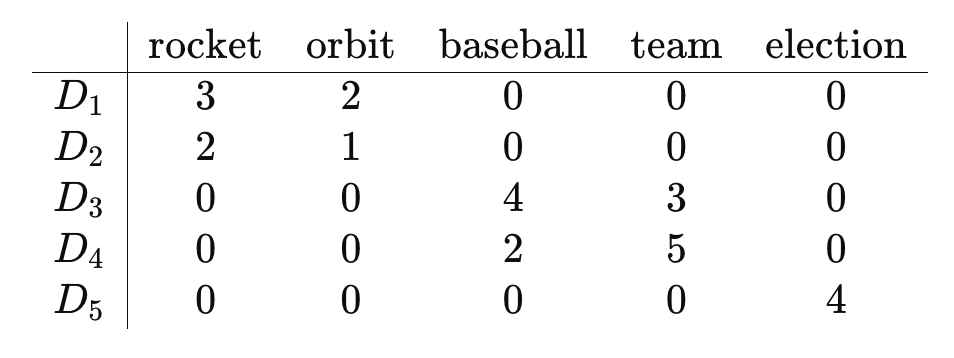
Topic modeling tries to discover the hidden structure behind this matrix.

How is SVD used for topic modelling?

When we apply truncated SVD to the document-term matrix, we write $X = U_k \Sigma_k V_k^T$. Here, $k$ is the number of latent dimensions/topics we want to keep. The important pieces are: $U_k \Sigma_k$ and $V_k^T$. The matrix $U_k \Sigma_k$ gives a low-dimensional representation of documents. Each document becomes a vector like: $[0.8,0.1,0.0,0.3]$ if we keep 4 components. This can be interpreted roughly as:

• Document 1 has strong component 1, weak component 2, almost no component 3, moderate component 4.

So documents that use similar words end up close together in the SVD space. On the other hand, the components become word patterns. The rows of $V_k^T$ show how strongly each word contributes to each component. For example, one component may have large weights for:

• rocket, nasa, orbit, planet, mission

So we may interpret that component as a “space” topic. Another component may have large weights for:

• baseball, team, pitcher, game, season

So we may interpret that as a “sports” topic. This method of using SVD for topic modeling is often called Latent Semantic Analysis, or LSA.

What is "latent" in latent semantic analysis?

The topics are not directly given in the data. The original data only contains words and documents. The topics are hidden, or latent, patterns discovered from word co-occurrence. For example, the words: rocket, orbit, nasa, planet, may not appear in every space-related document, but they often appear in similar contexts. SVD can capture this shared structure.

Is there a geometric interpretation?

Each document is originally a point in a very high-dimensional word space. For example, if the vocabulary has $20,000$ words, then each document is a point in $\mathbb{R}^{20000}$. SVD projects these documents into a smaller space $\mathbb{R}^k$. For example, $\mathbb{R}^{20000} \to \mathbb{R}^{100}$. The hope is that this smaller space captures major semantic patterns. Documents about similar topics should become closer together.

Why does SVD help?

SVD helps topic modeling because it can group related words and documents through shared patterns. For example, car, automobile, vehicle may not always appear together in the same document, but they may appear in similar contexts. SVD can partially capture this relationship. It can also reduce noise by ignoring smaller singular values. So instead of using every rare or noisy word, SVD keeps the strongest patterns of variation. The important limitation is that SVD components are not always clean topics. A component is a linear combination of words, and the weights can be positive or negative. So one component may mix multiple themes, such as:

• space words with positive weights
• sports words with negative weights

This can make interpretation harder. Also, SVD is not a probabilistic model. It does not directly model $\mathbf{Pr}[\text{topic} | \text{document}]$ or $\mathbf{Pr}[\text{word} | \text{topic}]$. It gives linear algebraic components, not probability distributions.

Are there other topic modeling methods?

Another common topic modeling method is Latent Dirichlet Allocation, or LDA. A rough comparison:

Method	Basic idea	Output
SVD / LSA	Matrix factorization	Latent components
LDA	Probabilistic generative model	Topic distributions
NMF	Nonnegative matrix factorization	Nonnegative topics

SVD is often fast and useful, but topics may be harder to interpret because components can have negative weights. NMF is often easier to interpret because it keeps nonnegative word-topic weights. LDA gives a probabilistic topic model, but it can be more complex to fit and tune.

Let's see LSA in action for our dateset.

tfidf_for_topics = TfidfVectorizer(stop_words="english", min_df=3, max_df=0.8)
X_topics = tfidf_for_topics.fit_transform(train.data)

svd_topics = TruncatedSVD(n_components=10, random_state=RANDOM_STATE)
X_lsa = svd_topics.fit_transform(X_topics)

terms = tfidf_for_topics.get_feature_names_out()

for i, comp in enumerate(svd_topics.components_):
    top_indices = comp.argsort()[-12:][::-1]
    top_terms = [terms[j] for j in top_indices]
    print(f"Component {i}: {top_terms}")

Here are some interesting questions to think about:

1. Do the components look like topics?
2. Which component seems related to space?
3. Which component seems related to baseball?
4. Are some components hard to interpret?
5. Why should we be careful when interpreting SVD components as topics?

11.3. SVD for image compression

A grayscale image can be represented as a matrix. SVD gives low-rank approximations of this matrix. A rank-$k$ approximation is: $$A_k = U_k \Sigma_k V_k^T.$$ Small values of $k$ use fewer numbers but give rougher images. Larger values of $k$ preserve more detail.

img = load_sample_image("china.jpg")

# Convert RGB image to grayscale using a simple luminance formula.
gray = (0.299 * img[:, :, 0] + 0.587 * img[:, :, 1] + 0.114 * img[:, :, 2]) / 255.0

plt.figure()
plt.imshow(gray, cmap="gray")
plt.title("Original grayscale image")
plt.axis("off")
plt.show()

print("Image matrix shape:", gray.shape)

U_img, S_img, VT_img = np.linalg.svd(gray, full_matrices=False)

for k in [5, 20, 50, 100]:
    approx = U_img[:, :k] @ np.diag(S_img[:k]) @ VT_img[:k, :]
    
    plt.figure()
    plt.imshow(approx, cmap="gray")
    plt.title(f"Rank-{k} approximation")
    plt.axis("off")
    plt.show()

plt.figure()
plt.plot(S_img[:100], marker="o")
plt.xlabel("Index")
plt.ylabel("Singular value")
plt.title("First 100 singular values of the image")
plt.grid(True)
plt.show()

Here are a few things to think about for image compression using SVD.

1. What happens to image quality as $k$ increases?
2. What visual information is captured by the first few singular values?
3. How many numbers are needed to store a rank-$k$ approximation of an $m \times n$ image?
4. Why is SVD useful for compression?

Here are some of the other methods for image compression:

• Lossless compression:
  • Run-Length Encoding, RLE
  • Huffman coding
  • Arithmetic coding
  • PNG-style compression
• Lossy compression:
  • JPEG compression
  • Wavelet compression
  • Vector quantization
  • Chroma subsampling
  • Transform coding
• Modern learned compression: These are modern neural methods that use something known as "autoencoders"

In summary, SVD is useful pedagogically and mathematically, but not the standard method for everyday image files.

11.4. SVD for noise reduction

Now we create a synthetic low-rank matrix and add noise. The clean matrix has true rank 5. After adding noise, the matrix is usually full-rank. Truncated SVD can recover the main signal by keeping only the largest singular values.

np.random.seed(RANDOM_STATE)

n, p, true_rank = 200, 100, 5
U_true = np.random.randn(n, true_rank)
V_true = np.random.randn(true_rank, p)

X_clean = U_true @ V_true
X_noisy = X_clean + 0.5 * np.random.randn(n, p)

print("Clean matrix shape:", X_clean.shape)

U_noisy, S_noisy, VT_noisy = np.linalg.svd(X_noisy, full_matrices=False)

errors_clean = []
errors_noisy = []
ks = range(1, 31)

for k in ks:
    X_hat = U_noisy[:, :k] @ np.diag(S_noisy[:k]) @ VT_noisy[:k, :]
    errors_clean.append(np.linalg.norm(X_clean - X_hat, "fro"))
    errors_noisy.append(np.linalg.norm(X_noisy - X_hat, "fro"))

plt.figure()
plt.plot(list(ks), errors_clean, marker="o")
plt.xlabel("Rank k")
plt.ylabel("Error compared with clean matrix")
plt.title("Denoising: reconstruction error against clean signal")
plt.grid(True)
plt.show()

plt.figure()
plt.plot(list(ks), errors_noisy, marker="o")
plt.xlabel("Rank k")
plt.ylabel("Error compared with noisy matrix")
plt.title("Fitting noisy data: reconstruction error against noisy matrix")
plt.grid(True)
plt.show()

11.5. SVD for recommendation-style latent factors

SVD is also connected to recommendation systems. A user-item matrix can be approximated by a low-rank matrix. Rows correspond to users and columns correspond to items. A low-rank approximation can reveal latent taste factors. This is a toy example. In real recommender systems, missing ratings should not simply be treated as zero.

R = np.array([
    [5, 4, 0, 0, 1],
    [4, 5, 0, 0, 1],
    [0, 0, 5, 4, 0],
    [0, 0, 4, 5, 0],
    [1, 1, 0, 0, 5]
], dtype=float)

ratings_df = pd.DataFrame(
    R,
    index=["User 1", "User 2", "User 3", "User 4", "User 5"],
    columns=["Item A", "Item B", "Item C", "Item D", "Item E"]
)

ratings_df

U_r, S_r, VT_r = np.linalg.svd(R, full_matrices=False)

k = 2
R_hat = U_r[:, :k] @ np.diag(S_r[:k]) @ VT_r[:k, :]

pd.DataFrame(
    np.round(R_hat, 2),
    index=ratings_df.index,
    columns=ratings_df.columns
)

user_embeddings = U_r[:, :2] @ np.diag(S_r[:2])
item_embeddings = VT_r[:2, :].T

plt.figure()
plt.scatter(user_embeddings[:, 0], user_embeddings[:, 1])
for i, label in enumerate(ratings_df.index):
    plt.text(user_embeddings[i, 0], user_embeddings[i, 1], label)
plt.xlabel("Latent dimension 1")
plt.ylabel("Latent dimension 2")
plt.title("User embeddings from rank-2 SVD")
plt.grid(True)
plt.show()

plt.figure()
plt.scatter(item_embeddings[:, 0], item_embeddings[:, 1])
for i, label in enumerate(ratings_df.columns):
    plt.text(item_embeddings[i, 0], item_embeddings[i, 1], label)
plt.xlabel("Latent dimension 1")
plt.ylabel("Latent dimension 2")
plt.title("Item embeddings from rank-2 SVD")
plt.grid(True)
plt.show()

Here are a few questions to think about:

1. Which users seem similar?
2. Which items seem similar?
3. What does the rank-2 approximation suggest about hidden preference patterns?
4. Why is it problematic to treat missing ratings as zero?
5. How might a real recommender system handle missing entries differently?

Here are some of the other ideas used for recommendation systems.

• User-based collaborative filtering: The idea is: "users with similar past behavior may like similar items." A typical similarity measure is cosine similarity: $sim(u, v) = \frac{r_u \cdot r_v}{||r_u|| \cdot ||r_v||}$, where $r_u$ and $r_v$ are rating vectors for users $u$ and $v$.
• Item-based collaborative filtering: This recommends items based on similar items. For example: "People who liked Movie A also liked Movie B." If a user likes Movie A, recommend similar movies. This is often more stable than user-based filtering because item similarities may change more slowly than user preferences.
• k-nearest neighbors recommendation: This is closely related to user-based or item-based collaborative filtering. For each user or item, find the $k$ nearest neighbors.
• Content-based recommendation: Content-based systems recommend items similar to what the user has liked before, based on item features. For movies, features might be: genre, actors, director, plot keywords, language, release year.
• Association rules: Association-rule mining finds patterns like: "If user bought A and B, they may also buy C."
• Popularity-based recommendation: This is the simplest method. Recommend the most popular items overall. This is often used as a baseline. It is also useful for new users because no personal history is needed. But it is not personalized.
• Demographic-based recommendation: This recommends based on user attributes such as: age group, location, language, profession, broad interests.
• Matrix factorization other than plain SVD:
  • Non-negative matrix factorization, NMF
  • Alternating least squares, ALS
  • Probabilistic matrix factorization
• Other methods include: Neural-network recommenders, Graph-based recommendation, Context-aware recommendation, Bandit-based recommendation

11.6. Project (100 points)

In this project, you are asked to use the concepts picked up in this lab to build a predictor for sentiment analysis using the Stanford Large Movie Review Dataset/IMDb dataset (link). It has 25,000 training reviews and 25,000 test reviews for binary sentiment classification, with labels positive/negative. The main question you will explore is:

Can Truncated SVD improve sentiment classification by compressing a high-dimensional TF-IDF representation into a smaller latent semantic representation?

The comparison should include:

• TF-IDF $\to$ Logistic Regression
• TF-IDF $\to$ Truncated SVD $\to$ Logistic Regression
• TF-IDF $\to$ k-NN
• TF-IDF $\to$ Truncated SVD $\to$ k-NN

You should use cross-validation to tune the hyperparameters, such as n_components (number of components in SVD) and n_neighbors (number of neighbors in KNN). Your analysis should also include Inspecting SVD “sentiment topics.” Some other questions your analysis should include are given below:

1. Does Truncated SVD improve k-NN sentiment classification?
2. Does Truncated SVD improve logistic regression?
3. How does the number of SVD components affect accuracy?
4. How does it affect training and prediction time?
5. Does explained variance predict classification accuracy?
6. Which model benefits more from SVD: k-NN or logistic regression?
7. Are SVD components interpretable as sentiment/topic directions?