ACOL106: Data Structures
(Recap: Python Module 3)
In the previous two modules, we covered Python programming basics that enabled us to write code for any computational task. As you start writing longer and more complex programs (or more appropriately programming projects) using only the programming concepts of the previous two modules, you realise that maintaining, updating, and debugging becomes very cumbersome. You start feeling the need to organise the code better by making it modular (i.e., defining small and more manageable code units designed for specific subtasks). This enables a better understanding of the code and easier management. For example, for debugging, we can try debugging individual modules. For updating and modifying, we can update the functionality of a few appropriate modules, while keeping the rest of the code intact. Distributing coding tasks to a team of programmers becomes easy since every programmer can be handed a few modules with clear specifications. The simplest tool for modularity in Python (and in most languages) is Functions.
1. Functions
In this section, we explore the creation of and use of functions in Python. As we did earlier, we draw a distinction between functions and methods. We use the general term function to describe a traditional, stateless function that is invoked without the context of a particular class or an instance of that class, such as sorted(data). We use the more specific term method to describe a member function that is invoked upon a specific object using an object-oriented message passing syntax, such as data.sort(). In this section, we only consider pure functions; methods will be explored with more general object-oriented principles in a subsequent module.We begin with an example to demonstrate the syntax for defining functions in Python. The following function counts the number of occurrences of a given target value within any form of iterable dataset.
    def count(data, target):
        n = 0
        for item in data:
            if item == target: # found a match
                n += 1
        return n
The first line, beginning with the keyword def, serves as the function’s signature. This establishes a new identifier as the name of the function (count, in this example), and it establishes the number of parameters that it expects, as well as names identifying those parameters (data and target, in this example). Unlike Java and C++, Python is a dynamically typed language, and therefore a Python signature does not designate the types of those parameters, nor the type (if any) of a return value. Those expectations should be stated in the function’s documentation and can be enforced within the body of the function, but misuse of a function will only be detected at run-time.
The remainder of the function definition is known as the body of the function. As is the case with control structures in Python, the body of a function is typically expressed as an indented block of code. Each time a function is called, Python creates a dedicated activation record that stores information relevant to the current call. This activation record includes what is known as a namespace to manage all identifiers that have local scope within the current call. The namespace includes the function’s parameters and any other identifiers that are defined locally within the body of the function. An identifier in the local scope of the function caller has no relation to any identifier with the same name in the caller’s scope (although identifiers in different scopes may be aliases to the same object). In our first example, the identifier n has scope that is local to the function call, as does the identifier item, which is established as the loop variable.
Let us experiment with the concepts introduced above.
def count(data, target):
    n = 0
    for item in data:
        if item == target: # found a match
            n += 1
    return n

name = "Harry Potter"
m = count(name, 'r')
print(m)
print(count([1, 2, 3, 4, 3, 5, 6, 3, 3, 4, 5, 3], 3))

n = 10 # Using an identifier that is also used within the function
print("n before function call = ", n)
print(count([1, 2, 3, 4, 3, 5, 6, 3, 3, 4, 5, 3], 3))
print("n after function call = ", n) #Checking if n gets updated when executing the function
3
5
n before function call =  10
5
n after function call =  10
Return statement
A return statement is used within the body of a function to indicate that the function should immediately cease execution, and that an expressed value should be returned to the caller. If a return statement is executed without an explicit argument, the None value is automatically returned. Likewise, None will be returned if the flow of control ever reaches the end of a function body without having executed a return statement. Often, a return statement will be the final command within the body of the function, as was the case in our earlier example of a count function. However, there can be multiple return statements in the same function, with conditional logic controlling which such command is executed, if any. As a further example, consider the following function that tests if a value exists in a sequence.
    def contains(data, target):
        for item in target:
            if item == target: # found a match
            return True
        return False
If the conditional within the loop body is ever satisfied, the return True statement is executed and the function immediately ends, with True designating that the target value was found. Conversely, if the for loop reaches its conclusion without ever finding the match, the final return False statement will be executed. Let's experiment with the above code.
def contains(data, target):
    for item in data:
        if item == target: # found a match
            return True
            print("This statement will never get printed")
    return False

print(contains("Harry potter", 'r'))
print(contains("Harry potter", 'z'))
True
False
Information passing
It is very important to have a clear understanding of the mechanism by which a programming language passes information to and from a function. In the context of a function signature, the identifiers used to describe the expected parameters are known as formal parameters, and the objects sent by the caller when invoking the function are the actual parameters. Parameter passing in Python follows the semantics of the standard assignment statement. When a function is invoked, each identifier that serves as a formal parameter is assigned, in the function’s local scope, to the respective actual parameter that is provided by the caller of the function.For example, consider the count function defined above and a call to this function m = count(name, 'r'). Just before the function body is executed, the actual parameters, name and 'r', are implicitly assigned to the formal parameters, data and target in the following manner:
    data = name
    target = 'r'
These assignment statements establish identifier data as an alias for name and target as a name for the string literal 'r'. (See Figure below)
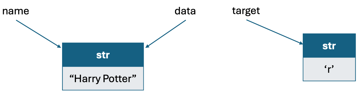
The communication of a return value from the function back to the caller is similarly implemented as an assignment. Therefore, with our sample invocation of m = count(name, 'r' ), the identifier m in the caller’s scope is assigned to the object that is identified as n in the return statement within our function body.
An advantage to Python’s mechanism for passing information to and from a function is that objects are not copied. This ensures that the invocation of a function is efficient, even in a case where a parameter or return value is a complex object. Let's experiment with some of the above concepts.
#The id() built-in function returns a unique integer that represents
#the identity of an object. This is essentially its memory address.

def count(data, target):
    print("(Inside function) ID of data = ", id(data))
    print("(Inside function) ID of target = ", id(target))
    n = 0
    for item in data:
        if item == target: # found a match
            n += 1
    print("(Inside function) ID of n = ", id(n))
    return n

name = 'Harry Potter'
t = 'r'
print("ID of name = ", id(name))
print("ID of t = ", id(t))
m = count(name, t)
print("ID of m = ", id(m))
ID of name =  4374578608
ID of t =  4329571056
(Inside function) ID of data =  4374578608
(Inside function) ID of target =  4329571056
(Inside function) ID of n =  4329056624
ID of m =  4329056624
Mutable parameters
Python’s parameter passing model has additional implications when a parameter is a mutable object. Because the formal parameter is an alias for the actual parameter, the body of the function may interact with the object in ways that change its state. Considering again a sample invocation of the count function:
    D = [1, 2, 3, 4, 3, 5, 6, 3, 3, 4, 5, 3]
    m = count(D, 3)
If the body of the function executes the command data.append(8)mark, the new entry is added to the
end of the list identified as data within the function, which is one and the same as the list known to the caller as D. As an aside, we note that reassigning a new value to a formal parameter with a function body, such as by setting data = [], does not alter the actual parameter; such a reassignment simply breaks the alias.Our hypothetical example of a count method that appends a new element to a list lacks common sense. There is no reason to expect such behavior, and it would be quite a poor design to have such an unexpected effect on the parameter. There are, however, many legitimate cases in which a function may be designed (and clearly documented) to modify the state of a parameter. As a concrete example, we present the following implementation of a method named scale whose primary purpose is to multiply all entries of a numeric data set by a given factor.
    def scale(data, factor):
        for j in range(len(data)):
            data[j] *= factor
Let's experiment with some of the above concepts.
def contains(data, target):
    for item in data:
        if item == target: # found a match
            data.append(target)# Appends target to data
            return True
    return False

D = [1, 2, 3]
print("D before checking 2", D)
contains(D, 2)
print("D after checking 2", D)
D before checking 2 [1, 2, 3]
D after checking 2 [1, 2, 3, 2]
Default parameter values
Python provides means for functions to support more than one possible calling signature. Such a function is said to be polymorphic (which is Greek for “many forms”). Most notably, functions can declare one or more default values for parameters, thereby allowing the caller to invoke a function with varying numbers of actual parameters. As an artificial example, if a function is declared with a signature def foo(a, b=15,c=27):, there are three parameters, the last two of which offer default values. A caller is welcome to send three actual parameters, as in foo(4, 12, 8), in which case the default values are not used. If, on the other hand, the caller only sends one parameter, foo(4), the function will execute with parameter values a=4, b=15, c=27. If a caller sends two parameters, they are assumed to be the first two, with the third being the default. Thus, foo(8, 20) executes with a=8, b=20, c=27. However, it is illegal to define a function with a signature such as bar(a, b=15, c) with b having a default value, yet not the subsequent c; if a default parameter value is present for one parameter, it must be present for all further parameters.For example, the typical use case for the count function may be to count the number of sentences in an input text. In such a case, it makes sense to use def count(data, target="."). Let's experiment with some of the above concepts.
def count(data, target="."):
    n = 0
    for item in data:
        if item == target: # found a match
            n += 1
    return n

text = """I give Pirrip as my father’s family name, on the authority of his
tombstone and my sister, Mrs Joe Gargery, who married the blacksmith. As
I never saw my father or my mother, and never saw any likeness of either of
them (for their days were long before the days of photographs), my first
fancies regarding what they were like were unreasonably derived from their
tombstones. The shape of the letters on my father’s, gave me an odd idea
that he was a square, stout, dark man, with curly black hair. From the
character and turn of the inscription, “Also Georgiana Wife of the Above,”
I drew a childish conclusion that my mother was freckled and sickly. To
five little stone lozenges, each about a foot and a half long, which
were arranged in a neat row beside their grave, and were sacred to the
memory of five little brothers of mine, who gave up trying to get a
living, exceedingly early in that universal struggle, I am indebted for
a belief I religiously entertained that they had all been born on their
backs with their hands in their trousers-pockets, and had never taken
them out in this state of existence.
"""
print(count(text)) #Counting sentences
print(count(text, '\n')) #Counting lines
print(count(text, ' ') + count(text, '\n')) #Counting words
# Technically, the above are not a very accurate way to count sentences and words,
# but are okay for getting estimates.
5
16
216
Keyword parameter
The traditional mechanism for matching the actual parameters sent by a caller to the formal parameters declared by the function signature is based on the concept of positional arguments. For example, with signature foo(a=10, b=20, c=30), parameters sent by the caller are matched, in the given order, to the formal parameters. An invocation of foo(5) indicates that a=5, while b and c are assigned their default values.Python supports an alternate mechanism for sending a parameter to a function known as a keyword argument. A keyword argument is specified by explicitly assigning an actual parameter to a formal parameter by name. For example, with the above definition of function foo, a call foo(c=5) will invoke the function with parameters a=10, b=20, c=5. A function’s author can require that certain parameters be sent only through the keyword-argument syntax. We will typically not define such functions. Let's experiment with the keyword parameter.
def foo(a=10, b=20, c=30):
    return([a, b, c])

print(foo(1, 2, 3))
print(foo(2, 1, 3))
print(foo(b=2))
print(foo(b=1, c=2, a=3))
[1, 2, 3]
[2, 1, 3]
[10, 2, 30]
[3, 1, 2]
Python's built-in functions
Python's built-in functions can be categorized according to their functionality as follows:- Input/Output: We have already seen some input/output functions.
- Character Encoding: ord and chr relate characters and their integer code points. For example, ord('A') is 65 and chr(65) is 'A' .
- Mathematics: abs, divmod, pow, round, and sum provide common mathematical functionality; an additional math module will be introduced later.
- Ordering: max and min apply to any data type that supports a notion of comparison, or to any collection of such values. Likewise, sorted can be used to produce an ordered list of elements drawn from any existing collection.
- Collections/Iterations: range generates a new sequence of numbers; len reports the length of any existing collection; functions reversed, all, any, and map operate on arbitrary iterations as well; iter and next provide a general framework for iteration through elements of a collection, and are discussed later.
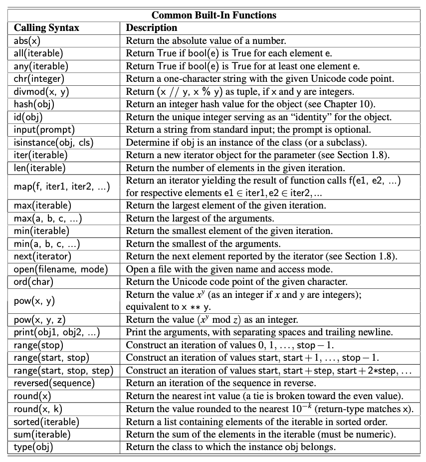
Try out some of these built-in functions below.
S = [1, 2, 3, 0]
print(all(S))
print(round(1.0013456, 4))
print(ord('#'))
L = [1, 2, 3, 4, 5, 6]
for i in reversed(L):print(i, end=", ")
False
1.0013
35
6, 5, 4, 3, 2, 1,
2. Iterators and genrators
In the section on control flow, we introduced the for-loop syntax beginning as:
for element in iterable:
and we noted that there are many types of objects in Python that qualify as being iterable. Basic container types, such as list, tuple, and set, qualify as iterable types. Furthermore, a string can produce an iteration of its characters, a dictionary can produce an iteration of its keys, and a file can produce an iteration of its lines. User-defined types may also support iteration. In Python, the mechanism for iteration is based upon the following conventions:
- An iterator is an object that manages an iteration through a series of values. If variable, i, identifies an iterator object, then each call to the built-in function, next(i), produces a subsequent element from the underlying series, with a StopIteration exception raised to indicate that there are no further elements. We shall learn about exceptions in the next section.
- An iterable is an object, obj, that produces an iterator via the syntax iter(obj).
More generally, it is possible to create multiple iterators based upon the same iterable object, with each iterator maintaining its own state of progress. However, iterators typically maintain their state with an indirect reference back to the original collection of elements. For example, calling iter(data) on a list instance produces an instance of the list_iterator class. That iterator does not store its own copy of the list of elements. Instead, it maintains a current index into the original list, representing the next element to be reported. Therefore, if the contents of the original list are modified after the iterator is constructed, but before the iteration is complete, the iterator will report the updated contents of the list.
Python also supports functions and classes that produce an implicit iterable series of values, that is, without constructing a data structure to store all of its values at once. For example, the call range(1000000) does not return a list of numbers; it returns a range object that is iterable. This object generates the million values one at a time, and only as needed. Such a lazy evaluation technique has a great advantage. In the case of range, it allows a loop of the form, for j in range(1000000):, to execute without setting aside memory for storing one million values. Also, if such a loop were to be interrupted in some fashion, no time would have been spent computing unused values of the range.
We see lazy evaluation used in many of Python’s libraries. For example, the dictionary class supports methods keys(), values(), and items(), which respectively produce a “view” of all keys, values, or (key, value) pairs within a dictionary. None of these methods produces an explicit list of results. Instead, the views that are produced are iterable objects based on the actual contents of the dictionary. An explicit list of values from such an iteration can be immediately constructed by calling the list class constructor with the iteration as a parameter. For example, the syntax list(range(1000)) produces a list instance with values from 0 to 999, while the syntax list(d.values()) produces a list that has elements based upon the current values of the dictionary d. We can similarly construct a tuple or set instance based upon a given iterable.
data = {'A':1, 'B':2, 'C':3}
i = iter(data)
j = data.values()
for k in i: print(k)
for k in j: print(k)
L = list(range(10))
print(L)
A
B
C
1
2
3
[0, 1, 2, 3, 4, 5, 6, 7, 8, 9]
Generators
In later modules, we will explain how to define a class whose instances serve as iterators. However, the most convenient technique for creating iterators in Python is through the use of generators. A generator is implemented with a syntax that is very similar to a function, but instead of returning values, a yield statement is executed to indicate each element of the series. As an example, consider the goal of determining all factors of a positive integer. For example, the number 100 has factors 1, 2, 4, 5, 10, 20, 25, 50, 100. A traditional function might produce and return a list containing all factors, implemented as:
    def factors(n):       # traditional function that computes factors
        results = []     # store factors in a new list
        for k in range(1,n+1):
            if n % k == 0: # divides evenly, thus k is a factor
                results.append(k) # add k to the list of factors
        return results     # return the entire list
In contrast, an implementation of a generator for computing those factors could be implemented as follows:
    def factors(n):         # generator that computes factors
        for k in range(1,n+1):
            if n % k == 0:  # divides evenly, thus k is a factor
                yield k     # yield this factor as next result
Notice the use of the keyword yield rather than return to indicate a result. This indicates to Python that we are defining a generator, rather than a traditional function. It is illegal to combine yield and return statements in the same implementation, other than a zero-argument return statement to cause a generator to end its execution. If a programmer writes a loop such as for factor in factors(100):, an instance of our generator is created. For each iteration of the loop, Python executes our procedure until a yield statement indicates the next value. At that point, the procedure is temporarily interrupted, only to be resumed when another value is requested. When the flow of control naturally reaches the end of our procedure (or a zero-argument return statement), a StopIteration exception is automatically raised. Although this particular example uses a single yield statement in the source code, a generator can rely on multiple yield statements in different constructs, with the generated series determined by the natural flow of control. For example, we can greatly improve the efficiency of our generator for computing factors of a number, n, by only testing values up to the square root of that number, while reporting the factor n//k that is associated with each k (unless n//k equals k). We might implement such a generator as follows:
    def factors(n): # generator that computes factors
        k = 1
        while k*k < n: # while k < sqrt(n)
            if n % k == 0:
                yield k
                yield n//k
            k += 1
        if k*k == n: # special case if n is a perfect square
            yield k
We should note that this generator differs from our first version in that the factors are not generated in strictly increasing order. For example, factors(100) generates the series 1,100,2,50,4,25,5,20,10.In closing, we wish to emphasize the benefits of lazy evaluation when using a generator rather than a traditional function. The results are only computed if requested, and the entire series need not reside in memory at one time. In fact, a generator can effectively produce an infinite series of values. As an example, the Fibonacci numbers form a classic mathematical sequence, starting with value 0, then value 1, and then each subsequent value being the sum of the two preceding values. Hence, the Fibonacci series begins as: 0,1,1,2,3,5,8,13,.... The following generator produces this infinite series.
    def fibonacci():
        a = 0
        b = 1
        while True:     # keep going...
            yield a     # report value, a, during this pass
            future = a + b
            a = b       # this will be next value reported
            b = future  # and subsequently this
Let's experiment with some of the above code.
def factors1(n):         # generator that computes factors
    for k in range(1,n+1):
        if n % k == 0:  # divides evenly, thus k is a factor
            yield k     # yield this factor as next result

def factors2(n): # generator that computes factors
    k = 1
    while k*k < n: # while k < sqrt(n)
        if n % k == 0:
            yield k
            yield n//k
        k += 1
    if k*k == n: # special case if n is a perfect square
        yield k

print("Factors of 200")
for i in factors1(200): print(i, end=", ")
print("\nFactors of 200")
for i in factors2(200): print(i, end=", ")


def fibonacci():
    a = 0
    b = 1
    while True:     # keep going...
        yield a     # report value, a, during this pass
        future = a + b
        a = b       # this will be next value reported
        b = future  # and subsequently this

print("\nPrinting Fibonacci sequence...")
j=0
for i in fibonacci():
    if(j>20):break
    print(i, end=", ")
    j +=1
Factors of 200
1, 2, 4, 5, 8, 10, 20, 25, 40, 50, 100, 200,
Factors of 200
1, 200, 2, 100, 4, 50, 5, 40, 8, 25, 10, 20,
Printing Fibonacci sequence...
0, 1, 1, 2, 3, 5, 8, 13, 21, 34, 55, 89, 144, 233, 377, 610, 987, 1597, 2584, 4181, 6765,
3. Exception handling
Exceptions are unexpected events that occur during the execution of a program. An exception might result from a logical error or an unanticipated situation. In Python, exceptions (also known as errors) are objects that are raised (or thrown) by code that encounters an unexpected circumstance. The Python interpreter can also raise an exception should it encounter an unexpected condition, like running out of memory. A raised error may be caught by a surrounding context that “handles” the exception in an appropriate fashion. If uncaught, an exception causes the interpreter to stop executing the program and to report an appropriate message to the console. In this section, we examine the most common error types in Python, the mechanism for catching and handling errors that have been raised, and the syntax for raising errors from within user-defined blocks of code.Common Exception types
Python includes a rich hierarchy of exception classes that designate various categories of errors; Table below shows many of those classes. The Exception class serves as a base class for most other error types. An instance of the various subclasses encodes details about a problem that has occurred. Several of these errors may be raised in exceptional cases by behaviors introduced in this chapter. For example, use of an undefined identifier in an expression causes a NameError, and errant use of the dot notation, as in foo.bar(), will generate an AttributeError if object foo does not support a member named bar.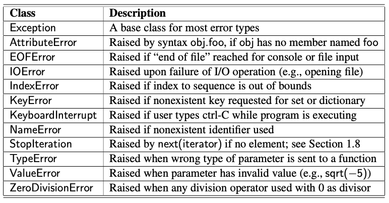
Sending the wrong number, type, or value of parameters to a function is another common cause for an exception. For example, a call to abs('hello') will raise a TypeError because the parameter is not numeric, and a call to abs(3, 5) will raise a TypeError because one parameter is expected. A ValueError is typically raised when the correct number and type of parameters are sent, but a value is illegitimate for the context of the function. For example, the int constructor accepts a string, as with int('137'), but a ValueError is raised if that string does not represent an integer, as with int('3.14') or int('hello').
Python’s sequence types (e.g., list, tuple, and str) raise an IndexError when syntax such as data[k] is used with an integer k that is not a valid index for the given sequence. Sets and dictionaries raise a KeyError when an attempt is made to access a nonexistent element. Let's try out some of the errors mentioned above.
# Please note that all the code snippets within Jupyter are executed in a sequence
# and not individually in isolation. So, if I print data, the dictionary data defined in
# a previous code segment will get printed
print(data)

# dat has not been defined within this module. Let's try to print it and see if it raises a NameError
#print(dat)

# We know that a dictionary does not support next method. Let's see if it causes AttributeError
# You will need to comment out the previous line
#print(data.next())

# Trying out other errors
#abs('Hello')
#int('3.14')
#data['D']
print(D)
D[5]
{'A': 1, 'B': 2, 'C': 3}
[1, 2, 3, 2]
---------------------------------------------------------------------------
IndexError                                Traceback (most recent call last)
Cell In[10], line 18
      6 # dat has not been defined within this module. Let's try to print it and see if it raises a NameError
      7 #print(dat)
      8
   (...)
     15 #int('3.14')
     16 #data['D']
     17 print(D)
---> 18 D[5]

IndexError: list index out of range
Raising an Exception
An exception is thrown by executing the raise statement, with an appropriate instance of an exception class as an argument that designates the problem. For example, if a function for computing a square root is sent a negative value as a parameter, it can raise an exception with the command:
raise ValueError('x cannot be negative')
This syntax raises a newly created instance of the ValueError class, with the error message serving as a parameter to the constructor. If this exception is not caught within the body of the function, the execution of the function immediately ceases, and the exception is propagated to the calling context (and possibly beyond).Exceptions have a lot of utility. Consider the following example. When checking the validity of parameters sent to a function, it is customary to first verify that a parameter is of an appropriate type and then to verify that it has an appropriate value. For example, the sqrt function in Python’s math library performs error-checking that might be implemented as follows:
    def sqrt(x):
        if not isinstance(x, (int, float)):
            raise TypeError('x must be numeric')
        elif x < 0:
            raise ValueError('x cannot be negative')
        # do the real work here...
Checking the type of an object can be performed at run-time using the built-in function, isinstance. In simplest form, isinstance(obj, cls) returns True if object, obj, is an instance of class, cls, or any subclass of that type. In the above example, a more general form is used with a tuple of allowable types indicated with the second parameter. After confirming that the parameter is numeric, the function enforces the expectation that the number be nonnegative, raising a ValueError otherwise.
How much error-checking to perform within a function is a matter of debate. Checking the type and value of each parameter demands additional execution time and, if taken to an extreme, seems counter to the nature of Python. Consider the built-in sum function, which computes the sum of a collection of numbers. An implementation with rigorous error-checking might be written as follows:
    def sum(values):
        if not isinstance(values, collections.Iterable):
            raise TypeError('parameter must be an iterable type')
        total = 0
        for v in values:
            if not isinstance(v, (int, float)):
                raise TypeError( elements must be numeric )
            total = total+ v
        return total
The abstract base class, collections.Iterable, includes all of Python’s iterable container types that guarantee support for the for-loop syntax (e.g., list, tuple, set); we see the use of modules, such as collections, in a subsequent section. Within the body of the for loop, each element is verified as numeric before being added to the total. A far more direct and clear implementation of this function can be written as follows:
    def sum(values):
        total = 0
        for v in values:
            total = total + v
        return total
Interestingly, this simple implementation performs exactly like Python’s built-in version of the function. Even without the explicit checks, appropriate exceptions are raised naturally by the code. In particular, if values is not an iterable type, the attempt to use the for-loop syntax raises a TypeError reporting that the object is not iterable. In the case when a user sends an iterable type that includes a nonnumerical element, such as sum([3.14, 'oops']), a TypeError is naturally raised by the evaluation of the expression total + v. The error message unsupported operand type(s) for +: ’float’ and ’str’ should be sufficiently informative to the caller. Perhaps slightly less obvious is the error that results from sum(['alpha', 'beta']). It will technically report a failed attempt to add an int and str, due to the initial evaluation of total + 'alpha', when total has been initialized to 0. We will favor the simpler implementations in the interest of clean presentation, performing minimal error-checking in most situations.
Catching an Exception
There are several philosophies regarding how to cope with possible exceptional cases when writing code. For example, if a division x/y is to be computed, there is a clear risk that a ZeroDivisionError will be raised when variable y has value 0. In an ideal situation, the logic of the program may dictate that y has a nonzero value, thereby removing the concern for error. However, for more complex code, or in a case where the value of y depends on some external input to the program, there remains some possibility of an error.One philosophy for managing exceptional cases is to “look before you leap.” The goal is to entirely avoid the possibility of an exception being raised through the use of a proactive conditional test. Revisiting our division example, we might avoid the offending situation by writing:
    if y != 0:
        ratio = x / y
    else:
        ... do something else ...
A second philosophy, often embraced by Python programmers, is that “it is easier to ask for forgiveness than it is to get permission.” This quote is attributed to Grace Hopper, an early pioneer in computer science. The sentiment is that we need not spend extra execution time safeguarding against every possible exceptional case, as long as there is a mechanism for coping with a problem after it arises. In Python, this philosophy is implemented using a try-except control structure. Revising our first example, the division operation can be guarded as follows:
    try:
        ratio = x / y
    except ZeroDivisionError:
        ... do something else ...
In this structure, the “try” block is the primary code to be executed. Although it is a single command in this example, it can more generally be a larger block of indented code. Following the try-block are one or more “except” cases, each with an identified error type and an indented block of code that should be executed if the
designated error is raised within the try-block.
The relative advantage of using a try-except structure is that the non-exceptional case runs efficiently, without extraneous checks for the exceptional condition. However, handling the exceptional case requires slightly more time when using a try-except structure than with a standard conditional statement. For this reason, the try-except clause is best used when there is reason to believe that the exceptional case is relatively unlikely, or when it is prohibitively expensive to proactively evaluate a condition to avoid the exception.
Exception handling is particularly useful when working with user input, or when reading from or writing to files, because such interactions are inherently less predictable. Earlier, we suggested the syntax, fp = open('sample.txt'), for opening a file with read access. That command may raise an IOError for a variety of reasons, such as a non-existent file or a lack of sufficient privilege for opening a file. It is significantly easier to attempt the command and catch the resulting error than it is to accurately predict whether the command will succeed.
We continue by demonstrating a few other forms of the try-except syntax. Exceptions are objects that can be examined when caught. To do so, an identifier must be established with a syntax as follows:
    try:
        fp = open('sample.txt')
    except IOError as e:
        print('Unable to open the file:', e)
In this case, the name e denotes the instance of the exception that was thrown, and printing it causes a detailed error message to be displayed (e.g., “file not found”).
A try-statement may handle more than one type of exception. For example, consider the following command from an earlier section:
age = int(input('Enter your age in years:'))
This command could fail for a variety of reasons. The call to input will raise an EOFError if the console input fails. If the call to input completes successfully, the int constructor raises a ValueError if the user has not entered characters representing a valid integer. If we want to handle two or more types of errors in the same way, we can use a single except-statement, as in the following example:
    age =−1 # an initially invalid choice
    while age <= 0:
        try:
            age = int(input('Enter your age in years:'))
            if age <= 0:
            print('Your age must be positive')
        except (ValueError, EOFError):
            print('Invalid response')
We use the tuple (ValueError, EOFError) to designate the types of errors that we wish to catch with the except clause. In this implementation, we catch either error, print a response, and continue with another pass of the enclosing while loop. We note that when an error is raised within the try-block, the remainder of that body is immediately skipped. In this example, if the exception arises within the call to input, or the subsequent call to the int constructor, the assignment to age never occurs, nor the message about needing a positive value. Because the value of age will be unchanged, the while loop will continue. If we preferred to have the while loop continue without printing the 'Invalid response' message, we could have written the exception clause as:
    except (ValueError, EOFError):
    pass
The keyword, pass, is a statement that does nothing, yet it can serve syntactically as a body of a control structure. In this way, we quietly catch the exception, thereby allowing the surrounding while loop to continue.
In order to provide different responses to different types of errors, we may use two or more except clauses as part of a try structure. In our previous example, an EOFError suggests a more insurmountable error than simply an errant value being entered. In that case, we might wish to provide a more specific error message, or perhaps to allow the exception to interrupt the loop and be propagated to a higher context. We could implement such behavior as follows:
    age =-1 # an initially invalid choice
    while age <= 0:
    try:
        age = int(input('Enter your age in years:'))
        if age <= 0:
            print('Your age must be positive')
    except ValueError:
        print('That is an invalid age specification')
    except EOFError:
        print('There was an unexpected error reading input.')
        raise # let's re-raise this exception
In this implementation, we have separate except clauses for the ValueError and EOFError cases. The body of the clause for handling an EOFError relies on another technique in Python. It uses the raise statement without any subsequent argument to re-raise the same exception that is currently being handled. This allows us to provide our own response to the exception, and then to interrupt the while loop and propagate the exception upward.
In closing, we note two additional features of try-except structures in Python. It is permissible to have a final except-clause without any identified error types, using syntax except:, to catch any other exceptions that occurred. However, this technique should be used sparingly, as it is difficult to suggest how to handle an error of an unknown type. A try-statement can have a finally clause, with a body of code that will always be executed in the standard or exceptional cases, even when an uncaught or re-raised exception occurs. That block is typically used for critical cleanup work, such as closing an open file. Let's experiment with some of these concepts.
try:
    fp = open('sample.txt')
except IOError as e:
    print('Unable to open the file:', e)
print("test")

def ask_age():
    age =-1 # an initially invalid choice
    while age <= 0:
        try:
            age = int(input('Enter your age in years:'))
            if age <= 0:
                print('Your age must be positive')
        except(ValueError, EOFError):
            print('Invalid response')

def ask_age1():
    age =-1 # an initially invalid choice
    while age <= 0:
        try:
            age = int(input('Enter your age in years:'))
            if age <= 0:
                print('Your age must be positive')
        except(ValueError, EOFError):
            pass

def ask_age2():
    age =-1 # an initially invalid choice
    while age <= 0:
        try:
            age = int(input('Enter your age in years:'))
            if age <= 0:
                print('Your age must be positive')
        except ValueError:
            print('That is an invalid age specification')
            raise
            print("After raise")
        except EOFError:
            print('There was an unexpected error reading input.')
            raise # let's re-raise this exception
    return age

#try:
#    age = ask_age2()
#except ValueError:
#    print('Something went wrong')
4. Additional Python conveniences
In this section, we introduce several features of Python that are particularly convenient for writing clean, concise code. Each of these syntaxes provide functionality that could otherwise be accomplished using functionality that we have introduced earlier in this chapter. However, at times, the new syntax is a more clear and direct expression of the logic.4.1 Conditional Expressions
Python supports a conditional expression syntax that can replace a simple control structure. The general syntax is an expression of the form:
expr1 if condition else expr2
This compound expression evaluates to expr1 if the condition is True, and otherwise evaluates to expr2. As an example, consider the goal of sending the absolute value of a variable, n, to a function (and without relying on the built-in abs function, for the sake of example). Using a traditional control structure, we might accomplish this as follows:
    if n >= 0:
        param = n
    else:
        param =−n
    result = foo(param) # call the function
With the conditional expression syntax, we can directly assign a value to variable param, as follows:
    param = n if n >= 0 else -n     # pick the appropriate value
    result = foo(param)             # call the function
In fact, there is no need to assign the compound expression to a variable. A conditional expression can itself serve as a parameter to the function, written as follows:
result = foo(n if n >= 0 else -n)
Sometimes, the mere shortening of source code is advantageous because it avoids the distraction of a more cumbersome control structure. However, we recommend that a conditional expression be used only when it improves the readability of the source code, and when the first of the two options is the more “natural” case,
given its prominence in the syntax. (We prefer to view the alternative value as more exceptional.) Let's experiment.
score = 40
print('Pass' if score >= 30 else 'Fail')
4.2 Comprehension sytax
A very common programming task is to produce one series of values based upon the processing of another series. Often, this task can be accomplished quite simply in Python using what is known as a comprehension syntax. We begin by demonstrating list comprehension, as this was the first form to be supported by Python. Its general form is as follows:
[ expression for value in iterable if condition ]
We note that both expression and condition may depend on value, and that the if-clause is optional. The evaluation of the comprehension is logically equivalent to the following traditional control structure for computing a resulting list:
    result = [ ]
    for value in iterable:
        if condition:
            result.append(expression)
As a concrete example, a list of the squares of the numbers from 1 to n, that is [1,4,9,16,25,... ,n^2], can be created by traditional means as follows:
    squares = []
    for k in range(1, n+1):
        squares.append(k*k)
With list comprehension, this logic is expressed as follows:
squares = [k*k for k in range(1, n+1)]
As a second example, an earlier section introduced the goal of producing a list of factors for an integer n. That task is accomplished with the following list comprehension:
factors = [k for k in range(1,n+1) if n % k == 0]
Python supports similar comprehension syntaxes that respectively produce a set, generator, or dictionary. We compare those syntaxes using our example for producing the squares of numbers.
    [ k*k for k in range(1, n+1) ]     # list comprehension
    { k*k for k in range(1, n+1) }     # set comprehension
    ( k*k for k in range(1, n+1) )     # generator comprehension
    { k : k*k for k in range(1, n+1) } # dictionary comprehension
The generator syntax is particularly attractive when results do not need to be stored in memory. For example, to compute the sum of the first n squares, the generator syntax total = sum(k*k for k in range(1, n+1)), is preferred to the use of an explicitly instantiated list comprehension as the parameter. Let's experiment.
# A short code for printing the prime numbers smaller than n
n = 100
primes = [k for k in range(1, n) if (True if all([False for j in range(2, k) if (k%j == 0)]) else False)]
print(len(primes))

sq1 = {k*k for k in range(1, n+1)}
print(sq1)

sq2 = (k*k for k in range(1, n+1))
print([n for n in sq2])

sq3 = {k : k*k for k in range(1, n+1)}
print([sq3[key] for key in sq3])
4.3 Packing and Unpacking of Sequences
Python provides two additional conveniences involving the treatment of tuples and other sequence types. The first is rather cosmetic. If a series of comma-separated expressions are given in a larger context, they will be treated as a single tuple, even if no enclosing parentheses are provided. For example, the assignment
data = 2, 4, 6, 8
results in identifier, data, being assigned to the tuple (2, 4, 6, 8). This behavior is called automatic packing of a tuple. One common use of packing in Python is when returning multiple values from a function. If the body of a function executes the command,
return x, y
it will be formally returning a single object that is the tuple (x, y).As a dual to the packing behavior, Python can automatically unpack a sequence, allowing one to assign a series of individual identifiers to the elements of a sequence. As an example, we can write
a, b, c, d = range(7, 11)
which has the effect of assigning a=7, b=8, c=9, and d=10, as those are the four values in the sequence returned by the call to range. For this syntax, the right-hand
side expression can be any iterable type, as long as the number of variables on the left-hand side is the same as the number of elements in the iteration.
This technique can be used to unpack tuples returned by a function. For example, the built-in function, divmod(a, b), returns the pair of values (a // b, a % b) associated with an integer division. Although the caller can consider the return value to be a single tuple, it is possible to write
quotient, remainder = divmod(a, b)
to separately identify the two entries of the returned tuple. This syntax can also be used in the context of a for loop, when iterating over a sequence of iterables, as in
for x, y in [ (7, 2), (5, 8), (6, 4) ]:
In this example, there will be three iterations of the loop. During the first pass, x=7 and y=2, and so on. This style of loop is quite commonly used to iterate through key-value pairs that are returned by the items() method of the dict class, as in:
for k, v in mapping.items():
Let's experiment with some of the above.
data = 1, 2, 3, 4, 5
print(data)

def maxmin(data):
    return max(data), min(data)

mm = maxmin(data)
print(mm)

a, b, c, d = range(7, 11)
print("a, b, c, d = ", a, b, c, d)

maximum, minimum = maxmin(data)
print("Max = ", maximum)
print("Min = ", minimum)

for x, y in [(7, 2), (5, 8), (6, 4)]:
    print([x, y])

sq3 = {k : k*k for k in range(1, 10)}
for k, v in sq3.items():
    print(k, v)
Simultaneous Assignments
The combination of automatic packing and unpacking forms a technique known as simultaneous assignment, whereby we explicitly assign a series of values to a series of identifiers, using a syntax:
x, y, z = 6, 2, 5
In effect, the right-hand side of this assignment is automatically packed into a tuple, and then automatically unpacked with its elements assigned to the three identifiers on the left-hand side.When using a simultaneous assignment, all of the expressions are evaluated on the right-hand side before any of the assignments are made to the left-hand variables. This is significant, as it provides a convenient means for swapping the values associated with two variables:
j, k = k, j
With this command, j will be assigned to the old value of k, and k will be assigned to the old value of j. Without simultaneous assignment, a swap typically requires more delicate use of a temporary variable, such as
    temp = j
    j = k
    k = temp
With the simultaneous assignment, the unnamed tuple representing the packed values on the right-hand side implicitly serves as the temporary variable when performing such a swap.
The use of simultaneous assignments can greatly simplify the presentation of code. As an example, we reconsider the generator defined earlier that produces the Fibonacci series. The original code requires separate initialization of variables a and b to begin the series. Within each pass of the loop, the goal was to reassign a and b, respectively, to the values of b and a+b. At the time, we accomplished this with a brief use of a third variable. With simultaneous assignments, that generator can be implemented more directly as follows:
    def fibonacci():
        a, b = 0, 1
        while True:
            yield a
            a, b = b, a+b
Let's try some of the above convenient statements.
i, j = 10, 20
print("i , j = ", i, ",", j)
i, j = j, i
print("i , j = ", i, ",", j)

def fibonacci():
        a, b = 0, 1
        while True:
            yield a
            a, b = b, a+b

for i in fibonacci():
    if (i > 100):break
    print(i, end=", ")
5. Scopes and Namespaces
When computing a sum with the syntax x + y in Python, the names x and y must have been previously associated with objects that serve as values; a NameError will be raised if no such definitions are found. The process of determining the value associated with an identifier is known as name resolution.Whenever an identifier is assigned to a value, that definition is made with a specific scope. Top-level assignments are typically made in what is known as a global scope. Assignments made within the body of a function typically have scope that is local to that function call. Therefore, an assignment, x = 5, within a function has no effect on the identifier, x, in the broader scope.
Each distinct scope in Python is represented using an abstraction known as a namespace. A namespace manages all identifiers that are currently defined in a given scope. The Figure below portrays two namespaces, one being that of a caller to the count function, and the other being the local namespace during the execution of that function. This is given in the code below:
    def count(data, target):
    n = 0
    for item in data:
        if item == target:
            n+=1
    return n
gpa = 3.56
major = 'CS'
grades = ['A-', 'B+', 'A-']
print("Number of A:", count(grades, 'A'))

In the above figure, the left namespace is the caller’s and the right namespace represents the local scope of the function.
Python implements a namespace with its own dictionary that maps each identifying string (e.g., 'n') to its associated value. Python provides several ways to examine a given namespace. The function dir reports the names of the identifiers in a given namespace (i.e., the keys of the dictionary), while the function vars returns the full dictionary. By default, calls to dir() and vars() report on the most locally enclosing namespace in which they are executed.
When an identifier is indicated in a command, Python searches a series of namespaces in the process of name resolution. First, the most locally enclosing scope is searched for a given name. If not found there, the next outer scope is searched, and so on. We will continue our examination of namespaces in a later section, when discussing Python’s treatment of object-orientation. We will see that each object has its own namespace to store its attributes, and that classes each have a namespace as well.
x = 10
def test():
    #x=20
    print(x)
test()
print(x)

def count(data, target):
    n = 0
    for item in data:
        if item == target:
            n+=1
    return n
gpa = 3.56
major = 'CS'
grades = ['A-', 'B+', 'A-']
print("Number of A: ", count(grades, 'A'))
First-Class Objects
In the terminology of programming languages, first-class objects are instances of a type that can be assigned to an identifier, passed as a parameter, or returned by a function. All of the data types we introduced in Module 1, such as int and list, are clearly first-class types in Python. In Python, functions and classes are also treated as first-class objects. For example, we could write the following:
    scream = print  # assign name ’scream’ to the function denoted as ’print’
    scream( Hello ) # call that function
In this case, we have not created a new function; we have simply defined scream as an alias for the existing print function. While there is little motivation for precisely this example, it demonstrates the mechanism that is used by Python to allow one function to be passed as a parameter to another. Within the keyword parameter section, we noted that the built-in function, max, accepts an optional keyword parameter to specify a non-default order when computing a maximum. For example, a caller can use the syntax max(a, b, key=abs) to determine which value has the larger absolute value. Within the body of that function, the formal parameter key is an identifier that will be assigned to the actual parameter, abs. In terms of namespaces, an assignment such as scream = print introduces the identifier scream into the current namespace, with its value being the object that represents the built-in function, print. The same mechanism is applied when a user-defined function is declared. For example, our count function beings with the following syntax:
    def count(data, target):
    ...
Such a declaration introduces the identifier count into the current namespace,
with the value being a function instance representing its implementation. In a similar
fashion, the name of a newly defined class is associated with a representation of
that class as its value. (Class definitions will be introduced in the next Module).
scream = print
scream("Hello")

a, b = -10, -20
print(max(a, b, key=abs))

def foo():
    def bar():
        print("bar")
    print("foo")
    bar()

foo()
#bar()
6. Modules and the Import Statement
We have already introduced many functions (e.g., max) and classes (e.g., list) that are defined within Python’s built-in namespace. Depending on the version of Python, there are approximately 130–150 definitions that were deemed significant enough to be included in that built-in namespace. Beyond the built-in definitions, the standard Python distribution includes perhaps tens of thousands of other values, functions, and classes that are organized in additional libraries, known as modules, that can be imported from within a program. As an example, we consider the math module. While the built-in namespace includes a few mathematical functions (e.g., abs, min, max, round), many more are relegated to the math module (e.g., sin, cos, sqrt). That module also defines approximate values for the mathematical constants, pi and e. Python’s import statement loads definitions from a module into the current namespace. One form of an import statement uses a syntax such as the following:
from math import pi, sqrt
This command adds both pi and sqrt, as defined in the math module, into the current namespace, allowing direct use of the identifier pi or a call of the function sqrt(2). If there are many definitions from the same module to be imported, an asterisk may be used as a wild card, as in from math import *, but this form should be used sparingly. The danger is that some of the names defined in the module may conflict with names already in the current namespace (or being imported from another module), and the import causes the new definitions to replace existing ones. Another approach that can be used to access many definitions from the same
module is to import the module itself, using a syntax such as: import math
Formally, this adds the identifier, math, to the current namespace, with the module as its value. (Modules are also first-class objects in Python.) Once imported, individual definitions from the module can be accessed using a fully-qualified name, such as math.pi or math.sqrt(2).
Creating a new module
To create a new module, one simply has to put the relevant definitions in a file named with a .py suffix. Those definitions can be imported from any other .py file within the same project directory. For example, if we were to put the definition of our count function into a file named utility.py, we could import that function using the syntax, from utility import count.It is worth noting that top-level commands with the module source code are executed when the module is first imported, almost as if the module were its own script. There is a special construct for embedding commands within the module that will be executed if the module is directly invoked as a script, but not when the module is imported from another script. Such commands should be placed in the body of a conditional statement of the following form,
if name == __main__ :
Using our hypothetical utility.py module as an example, such commands will be executed if the interpreter is started with the command python utility.py, but not when the utility module is imported into another context. This approach is often used to embed what are known as unit tests within the module; we will discuss unit testing in a later section. In the experiments below, assume that there is a utility.py file in the same directory with the following commands:
print("Always executed")

if __name__ == '__main__':
    print("Executed when run as script and not when imported")

def count1(data, target):
    return len([1 for item in data if item == target])
# Create a file named utility.py with the lines below uncommented
#print("Always executed")
#if __name__ == '__main__':
#    print("Executed when run as script and not when imported")
#def count1(data, target):
#    return len([1 for item in data if item == target])

from utility import count1

print(count1("This is a sentence", "s"))
Existing modules
The table below provides a summary of a few available modules that are relevant to a study of data structures. We have already discussed the math module briefly. In the remainder of this section, we highlight another module that is particularly important for some of the data structures and algorithms that we will study later in this book.
Pseudo-Random Number Generation
Python’s random module provides the ability to generate pseudo-random numbers, that is, numbers that are statistically random (but not necessarily truly random). A pseudo-random number generator uses a deterministic formula to generate the next number in a sequence based upon one or more past numbers that it has generated. Indeed, a simple yet popular pseudo-random number generator chooses its next number based solely on the most recently chosen number and some additional parameters using the following formula.
next = (a*current + b) % n
where a, b, and n are appropriately chosen integers. Python uses a more advanced technique known as a Mersenne Twister. It turns out that the sequences generated by these techniques can be proven to be statistically uniform, which is usually good enough for most applications requiring random numbers, such as games. For applications, such as computer security settings, where one needs unpredictable random sequences, this kind of formula should not be used. Instead, one should ideally sample from a source that is actually random, such as radio static coming from outer space.Since the next number in a pseudo-random generator is determined by the previous number(s), such a generator always needs a place to start, which is called its seed. The sequence of numbers generated for a given seed will always be the same. One common trick to get a different sequence each time a program is run is to use a seed that will be different for each run. For example, we could use some timed input from a user or the current system time in milliseconds.
Python’s random module provides support for pseudo-random number generation by defining a Random class; instances of that class serve as generators with independent state. This allows different aspects of a program to rely on their own pseudo-random number generator, so that calls to one generator do not affect the sequence of numbers produced by another. For convenience, all of the methods supported by the Random class are also supported as stand-alone functions of the random module (essentially using a single generator instance for all top-level calls).

Methods supported by instances of the Random class, and as top-level functions of the random module are given in the table above. Time for some experiments.
from random import *

print(random())
print(randint(1, 100))
L = [1, 2, 3, 4, 5]
shuffle(L)
print(L)

R1 = Random()
R2 = Random()
print(R1.randint(1, 100))
print(R2.randint(1, 100))
7. Module endnote
This completes the overview of most of the concepts of Python programming. What remains is Object Oriented Programmin (OOP), a programming paradigm that has several advantages when executing large programming projects. This will be covered in the next module.